import warnings
import sys
sys.path.insert(0, '..')

import arviz as az
import matplotlib.pyplot as plt
import numpy as np
import pandas as pd
import pymc as pm
import xarray as xr
from scipy import stats

az.style.use("arviz-variat")
az.rcParams["stats.ci_prob"] = 0.90
plt.rcParams["figure.dpi"] = 75
SEED = 7412Debugging a model: World Cup football
This notebook includes the code for the Bayesian Workflow book Chapter 23 Debugging a model: World Cup football.
1 World Cup 2014 team performance analysis
We use an item-response model such as described in the previous chapter to fit a model to estimate the abilities of the teams in the 2014 football World Cup. We use score differentials as data (ignoring the shoot-outs).
Game scores could be modelled with a discrete bivariate Poisson model, and score differences with Poisson difference models Karlis and Ntzoufras (2003), which are commonly used in analysis of sports data. But we’ll start with continuous models and discretized continuous models to illustrate how those can be compared, and eventually build also models using naturally discrete data models.
Load packages
from cmdstanpy import CmdStanModel, disable_logging
disable_logging()
from utils import print_stan
/home/osvaldo/anaconda3/envs/bwb/lib/python3.14/site-packages/tqdm/auto.py:21: TqdmWarning: IProgress not found. Please update jupyter and ipywidgets. See https://ipywidgets.readthedocs.io/en/stable/user_install.html
from .autonotebook import tqdm as notebook_tqdm2 Data
Data include 64 game results from World Cup 2014 and Soccer Power Index that was available on the internet a month before the tournament Silver (2014). We took the rankings, with Brazil at the top (getting a score of 32) and Australia at the bottom (with a score of 1), and then for simplicity in interpretation of the parameters we rescaled these to have mean 0 and standard deviation 1/2, to get “prior scores” that ranged from \(-0.83\) to \(+0.83\).
powerindex = pd.read_csv("data/soccerpowerindex.csv")
rev_index = powerindex["index"].values[::-1]
powerindex["prior_score"] = (rev_index - rev_index.mean()) / rev_index.std(ddof=1) / 2
teamnames = powerindex["team"].values

worldcup = pd.read_csv("data/worldcup2014.csv")
team_to_idx = {team: i + 1 for i, team in enumerate(teamnames)}
worldcup["team_1"] = worldcup["team1"].map(team_to_idx)
worldcup["team_2"] = worldcup["team2"].map(team_to_idx)

N_games = len(worldcup)
gamenames = [
    f"{teamnames[t1 - 1]} vs. {teamnames[t2 - 1]}"
    for t1, t2 in zip(worldcup["team_1"], worldcup["team_2"])
][::-1]

dif = worldcup["score1"].values - worldcup["score2"].values
sqrt_dif = np.sign(dif) * np.sqrt(np.abs(dif))
sqrt_dif_fixed = 2 * np.sign(dif) * np.sqrt(np.abs(dif))
2.1 Data for Stan
stan_data = {
    "N_teams": len(powerindex),
    "N_games": N_games,
    "team_1": worldcup["team_1"].values.tolist(),
    "team_2": worldcup["team_2"].values.tolist(),
    "score_1": worldcup["score1"].values.tolist(),
    "score_2": worldcup["score2"].values.tolist(),
    "prior_score": powerindex["prior_score"].values.tolist(),
    "df": 7,
}
3 First model
The first model uses Student’s \(t\) for square root of score difference. It’s not particularly well justified model, but that is what Andrew first thought and it turned out to be useful for illustration.
The model structure is as follows: if game \(i\) has teams \(j_1\) and team \(j_2\) playing, and they score \(z_1\) and \(z_2\) goals, respectively, then the data point for this game is \(y_i = \mbox{sign}(z_1-z_2)*\sqrt{|z_1-z_2|}\), and the data model is: \(y_i \sim \mbox{normal}(a_{j_1[i]}-a_{j_2[i]}, \sigma_y)\), where \(a_{j_1}\) and \(a_{j_2}\) are the ability parameters (to use psychometrics jargon) for the two teams and \(\sigma_y\) is a scale parameter estimated from the data.
\[ y_i \sim \mbox{t}_{\nu}(a_{j_1[i]}-a_{j_2[i]}, \sigma_y), \] setting the degrees of freedom to \(\nu=7\).
Stan model
model_1 = CmdStanModel(stan_file="worldcup_first_try.stan")
print_stan(model_1)
/* This program has a mistake in it, as will be explained later */
data {
int N_teams;
int N_games;
vector[N_teams] prior_score;
array[N_games] int team_1;
array[N_games] int team_2;
vector[N_games] score_1;
vector[N_games] score_2;
real df;
}
transformed data {
vector[N_games] dif = score_1 - score_2;
vector[N_games] sqrt_dif;
for (i in 1:N_games) {
sqrt_dif[i] = (step(dif[i]) - 0.5) * sqrt(abs(dif[i]));
}
}
parameters {
vector[N_teams] alpha;
real b;
real<lower=0> sigma_a;
real<lower=0> sigma_y;
}
transformed parameters {
vector[N_teams] a = b * prior_score + sigma_a * alpha;
}
model {
alpha ~ normal(0, 1);
b ~ normal(0, 1);
sigma_a ~ normal(0, 1);
sigma_y ~ normal(0, 1);
sqrt_dif ~ student_t(df, a[team_1] - a[team_2], sigma_y);
}Fit the model and show the results
fit_1 = model_1.sample(data=stan_data, seed=SEED, show_progress=False)idata_1 = az.from_cmdstanpy(fit_1, coords={"a_dim_0": teamnames})
idata_1.posterior.ds = idata_1.posterior.ds.rename({
"a_dim_0": "teams",
})
az.summary(idata_1, var_names=["a", "b", "sigma_a", "sigma_y"])| mean | sd | eti90_lb | eti90_ub | ess_bulk | ess_tail | r_hat | mcse_mean | mcse_sd | |
|---|---|---|---|---|---|---|---|---|---|
| a[Bresil] | 0.288 | 0.144 | 0.038 | 0.51 | 3635 | 3288 | 1.00 | 0.0024 | 0.002 |
| a[Argentine] | 0.368 | 0.122 | 0.17 | 0.57 | 5423 | 3108 | 1.00 | 0.0017 | 0.0013 |
| a[Allemagne] | 0.488 | 0.159 | 0.25 | 0.77 | 1874 | 2439 | 1.00 | 0.0037 | 0.0027 |
| a[Espagne] | 0.163 | 0.176 | -0.15 | 0.42 | 2291 | 2691 | 1.00 | 0.0038 | 0.0029 |
| a[Chili] | 0.273 | 0.147 | 0.025 | 0.51 | 6151 | 2610 | 1.00 | 0.0019 | 0.0015 |
| a[France] | 0.302 | 0.138 | 0.08 | 0.53 | 4669 | 3198 | 1.00 | 0.002 | 0.0016 |
| a[Colombie] | 0.336 | 0.143 | 0.12 | 0.59 | 2605 | 3279 | 1.00 | 0.0028 | 0.0021 |
| a[Uruguay] | 0.141 | 0.149 | -0.12 | 0.37 | 4198 | 2961 | 1.00 | 0.0023 | 0.0019 |
| a[Angleterre] | 0.032 | 0.169 | -0.27 | 0.27 | 2054 | 3208 | 1.00 | 0.0037 | 0.0031 |
| a[Belgique] | 0.204 | 0.134 | -0.0046 | 0.44 | 4716 | 3226 | 1.00 | 0.002 | 0.0016 |
| a[Pays-Bas] | 0.336 | 0.164 | 0.098 | 0.62 | 1402 | 1884 | 1.00 | 0.0043 | 0.003 |
| a[Bosnie] | 0.047 | 0.157 | -0.24 | 0.28 | 4995 | 3086 | 1.00 | 0.0023 | 0.0019 |
| a[Equateur] | 0.055 | 0.147 | -0.2 | 0.29 | 5670 | 2905 | 1.00 | 0.002 | 0.0018 |
| a[Portugal] | 0.028 | 0.153 | -0.23 | 0.27 | 5348 | 2935 | 1.00 | 0.0021 | 0.0018 |
| a[Coted'Ivoire] | -0.029 | 0.154 | -0.3 | 0.2 | 4191 | 2931 | 1.00 | 0.0023 | 0.0019 |
| a[Russie] | -0.076 | 0.149 | -0.34 | 0.15 | 3871 | 3015 | 1.00 | 0.0024 | 0.0019 |
| a[Italie] | -0.053 | 0.153 | -0.32 | 0.19 | 5184 | 3050 | 1.00 | 0.0022 | 0.0019 |
| a[Suisse] | 0.003 | 0.141 | -0.22 | 0.24 | 5547 | 3019 | 1.00 | 0.0019 | 0.0016 |
| a[Etats-Unis] | -0.026 | 0.141 | -0.25 | 0.22 | 4618 | 2344 | 1.00 | 0.0021 | 0.0018 |
| a[Mexique] | 0.012 | 0.145 | -0.2 | 0.26 | 2964 | 3057 | 1.00 | 0.0027 | 0.0021 |
| a[Ghana] | -0.136 | 0.152 | -0.39 | 0.11 | 5658 | 2932 | 1.00 | 0.002 | 0.0018 |
| a[Grece] | -0.12 | 0.139 | -0.34 | 0.12 | 5384 | 2781 | 1.00 | 0.0019 | 0.0016 |
| a[Croatie] | -0.182 | 0.157 | -0.45 | 0.072 | 5916 | 2832 | 1.00 | 0.0021 | 0.0018 |
| a[Nigeria] | -0.156 | 0.139 | -0.38 | 0.091 | 5542 | 3478 | 1.00 | 0.0019 | 0.0016 |
| a[Coree] | -0.261 | 0.152 | -0.53 | -0.027 | 4575 | 3163 | 1.00 | 0.0023 | 0.0019 |
| a[CostaRica] | -0.02 | 0.176 | -0.27 | 0.29 | 1654 | 2718 | 1.00 | 0.0043 | 0.003 |
| a[Japon] | -0.296 | 0.15 | -0.55 | -0.054 | 5286 | 2701 | 1.00 | 0.0021 | 0.0017 |
| a[Cameroun] | -0.413 | 0.169 | -0.71 | -0.17 | 2300 | 2599 | 1.00 | 0.0035 | 0.0029 |
| a[Iran] | -0.303 | 0.145 | -0.54 | -0.06 | 5805 | 3223 | 1.00 | 0.0019 | 0.0016 |
| a[Honduras] | -0.419 | 0.159 | -0.7 | -0.19 | 2997 | 3085 | 1.00 | 0.0029 | 0.0023 |
| a[Algerie] | -0.217 | 0.163 | -0.45 | 0.078 | 2416 | 2768 | 1.00 | 0.0033 | 0.0026 |
| a[Australie] | -0.389 | 0.15 | -0.64 | -0.15 | 6946 | 3316 | 1.00 | 0.0018 | 0.0015 |
| b | 0.449 | 0.101 | 0.28 | 0.61 | 3089 | 2721 | 1.00 | 0.0018 | 0.0015 |
| sigma_a | 0.17 | 0.075 | 0.037 | 0.29 | 776 | 1014 | 1.00 | 0.0027 | 0.0018 |
| sigma_y | 0.42 | 0.053 | 0.34 | 0.51 | 1700 | 1869 | 1.00 | 0.0013 | 0.00097 |
pc = az.plot_forest(idata_1, var_names=["a"], combined=True, labels=["teams"])
pc.add_title("Team quality estimate with 90% intervals")
pc.coords = {"column": "forest"}
az.add_lines(pc, values=0)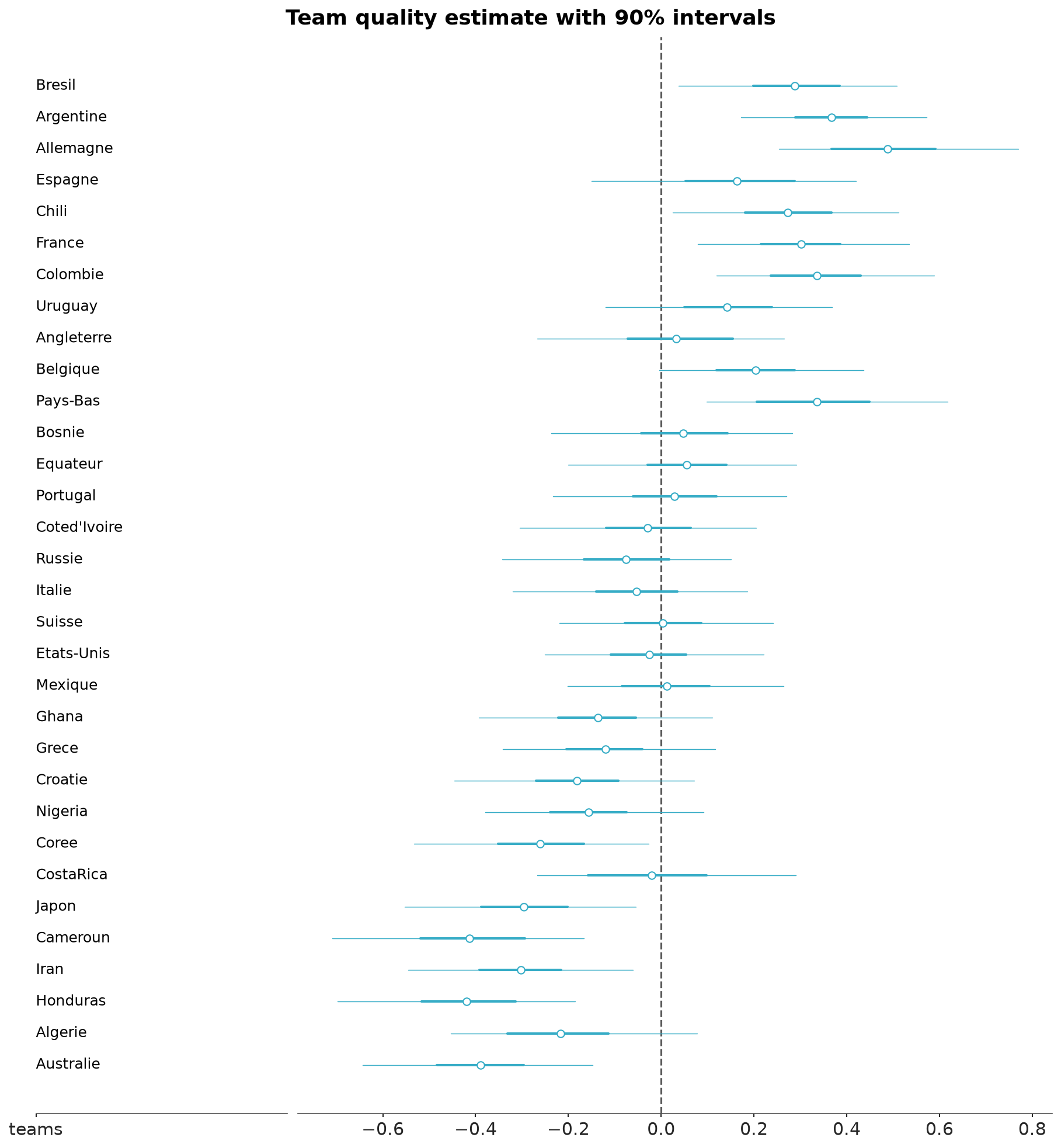
3.1 Check fit of the first model
model_1_rep = CmdStanModel(stan_file="worldcup_with_replication.stan")
print_stan(model_1_rep)
/* This program has a mistake in it, as will be explained later */
data {
int N_teams;
int N_games;
vector[N_teams] prior_score;
array[N_games] int team_1;
array[N_games] int team_2;
vector[N_games] score_1;
vector[N_games] score_2;
real df;
}
transformed data {
vector[N_games] dif = score_1 - score_2;
vector[N_games] sqrt_dif;
for (i in 1:N_games) {
sqrt_dif[i] = (step(dif[i]) - 0.5)*sqrt(abs(dif[i]));
}
}
parameters {
vector[N_teams] alpha;
real b;
real<lower=0> sigma_a;
real<lower=0> sigma_y;
}
transformed parameters {
vector[N_teams] a = b * prior_score + sigma_a * alpha;
}
model {
alpha ~ normal(0, 1);
b ~ normal(0, 1);
sigma_a ~ normal(0, 1);
sigma_y ~ normal(0, 1);
sqrt_dif ~ student_t(df, a[team_1] - a[team_2], sigma_y);
}
generated quantities {
vector[N_games] y_rep;
vector[N_games] y_rep_original_scale;
for (n in 1:N_games) {
y_rep[n] = student_t_rng(df, a[team_1[n]] - a[team_2[n]], sigma_y);
}
y_rep_original_scale = y_rep .* abs(y_rep);
}fit_1_rep = model_1_rep.sample(data=stan_data, seed=SEED, show_progress=False)idata_1_rep = az.from_cmdstanpy(
fit_1_rep,
posterior_predictive="y_rep_original_scale",
observed_data={"dif": dif},
coords={"y_rep_original_scale_dim_0": gamenames,
"dif_dim_0": gamenames}
)
idata_1_rep.posterior_predictive.ds = idata_1_rep.posterior_predictive.ds.rename({
"y_rep_original_scale": "dif",
"y_rep_original_scale_dim_0": "Games"
})
pc = az.plot_forest(
idata_1_rep,
group="posterior_predictive",
combined=True,
visuals={"trunk": False},
labels=["Games"],
)
pc.map(
az.visuals.scatter_x,
"observations",
data=idata_1_rep.observed_data.ds,
coords={"column": "forest"},
color="C1",
)
pc.add_title("Game score differentials\ncompared to 90% predictive interval")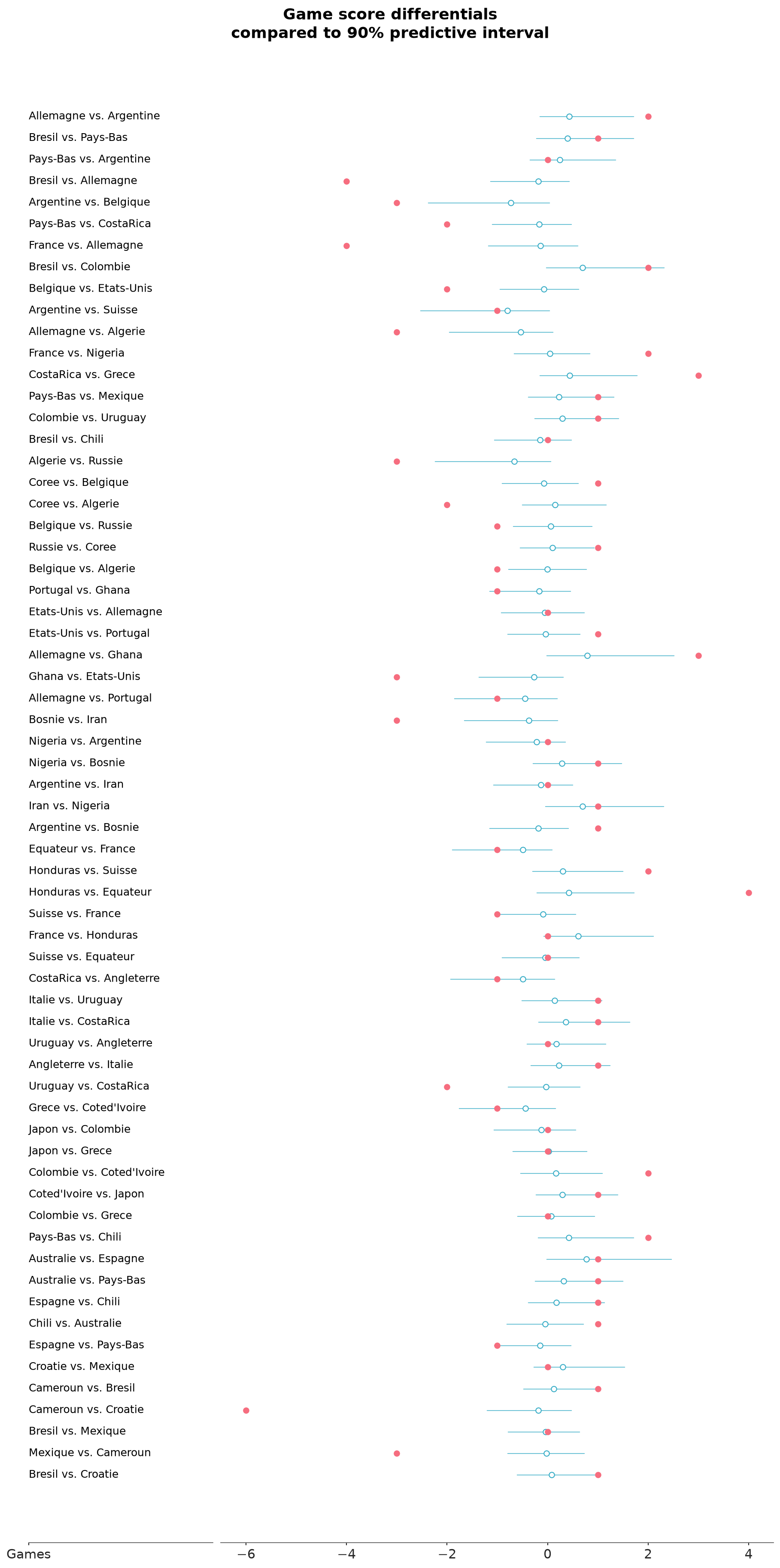
4 Second model without sqrt transformation
model_2 = CmdStanModel(stan_file="worldcup_no_sqrt.stan")
print_stan(model_2)
data {
int N_teams;
int N_games;
vector[N_teams] prior_score;
array[N_games] int team_1;
array[N_games] int team_2;
vector[N_games] score_1;
vector[N_games] score_2;
real df;
}
transformed data {
vector[N_games] dif = score_1 - score_2;
}
parameters {
vector[N_teams] alpha;
real b;
real<lower=0> sigma_a;
real<lower=0> sigma_y;
}
transformed parameters {
vector[N_teams] a = b * prior_score + sigma_a * alpha;
}
model {
alpha ~ normal(0, 1);
b ~ normal(0, 1);
sigma_a ~ normal(0, 1);
sigma_y ~ normal(0, 1);
dif ~ student_t(df, a[team_1] - a[team_2], sigma_y);
}
generated quantities {
vector[N_games] y_rep;
for (n in 1:N_games) {
y_rep[n] = student_t_rng(df, a[team_1[n]] - a[team_2[n]], sigma_y);
}
}fit_2 = model_2.sample(data=stan_data, seed=SEED, show_progress=False)idata_2 = az.from_cmdstanpy(fit_2, coords={"a_dim_0": teamnames})
idata_2.posterior.ds = idata_2.posterior.ds.rename({
"a_dim_0": "teams",
})
az.summary(idata_2, var_names=["a", "b", "sigma_a", "sigma_y"])| mean | sd | eti90_lb | eti90_ub | ess_bulk | ess_tail | r_hat | mcse_mean | mcse_sd | |
|---|---|---|---|---|---|---|---|---|---|
| a[Bresil] | 0.8 | 0.37 | 0.13 | 1.4 | 3756 | 2737 | 1.00 | 0.0062 | 0.0051 |
| a[Argentine] | 0.844 | 0.332 | 0.3 | 1.4 | 6516 | 3531 | 1.00 | 0.0041 | 0.0034 |
| a[Allemagne] | 1.08 | 0.41 | 0.5 | 1.8 | 2496 | 3218 | 1.00 | 0.0084 | 0.0069 |
| a[Espagne] | 0.53 | 0.45 | -0.34 | 1.2 | 2558 | 2383 | 1.00 | 0.0092 | 0.0085 |
| a[Chili] | 0.7 | 0.384 | 0.074 | 1.3 | 5101 | 2845 | 1.00 | 0.0055 | 0.0048 |
| a[France] | 0.81 | 0.37 | 0.29 | 1.5 | 3263 | 3222 | 1.00 | 0.0065 | 0.0054 |
| a[Colombie] | 0.85 | 0.38 | 0.32 | 1.6 | 2552 | 3021 | 1.00 | 0.0076 | 0.006 |
| a[Uruguay] | 0.36 | 0.38 | -0.32 | 0.92 | 3786 | 3034 | 1.00 | 0.0063 | 0.006 |
| a[Angleterre] | 0.21 | 0.4 | -0.53 | 0.78 | 2370 | 2614 | 1.00 | 0.0084 | 0.0078 |
| a[Belgique] | 0.421 | 0.323 | -0.089 | 0.98 | 5105 | 3363 | 1.00 | 0.0046 | 0.0043 |
| a[Pays-Bas] | 0.7 | 0.43 | 0.17 | 1.5 | 1734 | 2647 | 1.00 | 0.01 | 0.0083 |
| a[Bosnie] | 0.19 | 0.377 | -0.45 | 0.81 | 5082 | 3383 | 1.00 | 0.0052 | 0.0049 |
| a[Equateur] | 0.144 | 0.362 | -0.48 | 0.72 | 5697 | 3025 | 1.00 | 0.0048 | 0.0046 |
| a[Portugal] | 0.03 | 0.37 | -0.65 | 0.55 | 4460 | 2767 | 1.00 | 0.0058 | 0.0056 |
| a[Coted'Ivoire] | -0 | 0.345 | -0.63 | 0.53 | 4124 | 2844 | 1.00 | 0.0054 | 0.0049 |
| a[Russie] | -0.1 | 0.36 | -0.76 | 0.43 | 3891 | 3037 | 1.00 | 0.0058 | 0.0052 |
| a[Italie] | -0.08 | 0.35 | -0.69 | 0.48 | 4704 | 2797 | 1.00 | 0.0052 | 0.0051 |
| a[Suisse] | -0.02 | 0.36 | -0.56 | 0.61 | 4616 | 2731 | 1.00 | 0.0054 | 0.0051 |
| a[Etats-Unis] | -0.09 | 0.34 | -0.61 | 0.5 | 4543 | 3092 | 1.00 | 0.0051 | 0.0049 |
| a[Mexique] | -0.02 | 0.37 | -0.53 | 0.64 | 3115 | 2914 | 1.00 | 0.0067 | 0.0064 |
| a[Ghana] | -0.29 | 0.38 | -0.92 | 0.34 | 4373 | 2747 | 1.00 | 0.0058 | 0.0056 |
| a[Grece] | -0.35 | 0.354 | -0.94 | 0.24 | 5316 | 2995 | 1.00 | 0.005 | 0.0047 |
| a[Croatie] | -0.42 | 0.39 | -1.1 | 0.22 | 4615 | 2952 | 1.00 | 0.0058 | 0.0053 |
| a[Nigeria] | -0.4 | 0.36 | -0.98 | 0.23 | 5205 | 2938 | 1.00 | 0.0051 | 0.005 |
| a[Coree] | -0.6 | 0.38 | -1.3 | -0.018 | 4538 | 2733 | 1.00 | 0.0058 | 0.0053 |
| a[CostaRica] | -0.21 | 0.43 | -0.78 | 0.6 | 1942 | 2840 | 1.00 | 0.0098 | 0.0079 |
| a[Japon] | -0.73 | 0.39 | -1.4 | -0.14 | 4841 | 3079 | 1.00 | 0.0056 | 0.0052 |
| a[Cameroun] | -0.98 | 0.45 | -1.8 | -0.37 | 2458 | 2736 | 1.00 | 0.0092 | 0.0086 |
| a[Iran] | -0.75 | 0.38 | -1.4 | -0.13 | 4785 | 2136 | 1.00 | 0.0056 | 0.0052 |
| a[Honduras] | -1.05 | 0.42 | -1.8 | -0.44 | 3357 | 3157 | 1.00 | 0.0074 | 0.0064 |
| a[Algerie] | -0.6 | 0.43 | -1.2 | 0.18 | 2216 | 2543 | 1.00 | 0.0093 | 0.0079 |
| a[Australie] | -1 | 0.41 | -1.7 | -0.35 | 4655 | 3081 | 1.00 | 0.0058 | 0.0054 |
| b | 1.115 | 0.275 | 0.66 | 1.6 | 3286 | 2593 | 1.00 | 0.0048 | 0.0035 |
| sigma_a | 0.37 | 0.209 | 0.047 | 0.73 | 932 | 1271 | 1.01 | 0.0067 | 0.0045 |
| sigma_y | 1.289 | 0.152 | 1.1 | 1.6 | 2703 | 2432 | 1.00 | 0.0029 | 0.0022 |
pc = az.plot_forest(idata_2, var_names=["a"], combined=True, labels=["teams"])
pc.add_title("Team quality estimate with 90% intervals\n(model with no square root)")
pc.coords = {"column": "forest"}
az.add_lines(pc, values=0)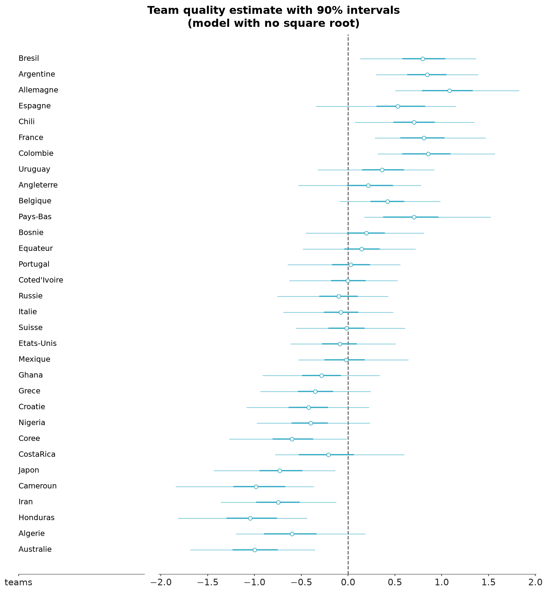
4.1 Check fit of the second model to data
idata_2_rep = az.from_cmdstanpy(
    fit_2,
    posterior_predictive="y_rep",
    observed_data={"dif": dif},
    coords={"y_rep_dim_0": gamenames, "dif_dim_0": gamenames}
)
idata_2_rep.posterior_predictive.ds = idata_2_rep.posterior_predictive.ds.rename({
    "y_rep": "dif",
    "y_rep_dim_0": "Games"
})

pc = az.plot_forest(
    idata_2_rep,
    group="posterior_predictive",
    combined=True,
    visuals={"trunk": False},
    labels=["Games"],
)
pc.map(
    az.visuals.scatter_x,
    "observations",
    data=idata_2_rep.observed_data.ds,
    coords={"column": "forest"},
    color="C1",
)
pc.add_title("Game score differentials\ncompared to 90% predictive interval")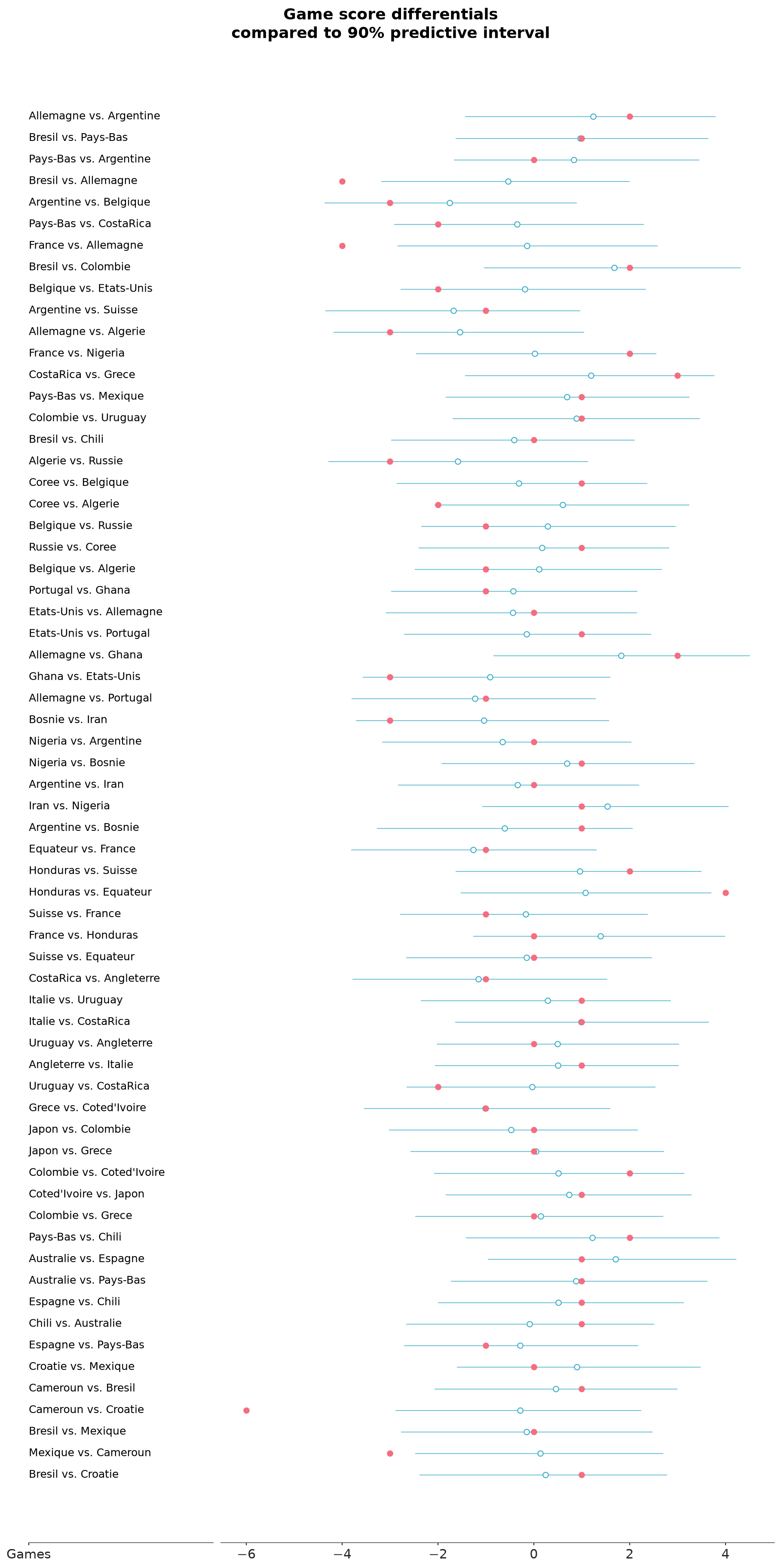
5 Fix the first model
model_3 = CmdStanModel(stan_file="worldcup_fixed.stan")
print_stan(model_3)
/* The error in the transformed data block has been fixed */
data {
int N_teams;
int N_games;
vector[N_teams] prior_score;
array[N_games] int team_1;
array[N_games] int team_2;
vector[N_games] score_1;
vector[N_games] score_2;
real df;
}
transformed data {
vector[N_games] dif = score_1 - score_2;
vector[N_games] sqrt_dif;
for (i in 1:N_games){
sqrt_dif[i] = 2 * (step(dif[i]) - 0.5) * sqrt(abs(dif[i]));
}
}
parameters {
vector[N_teams] alpha;
real b;
real<lower=0> sigma_a;
real<lower=0> sigma_y;
}
transformed parameters {
vector[N_teams] a = b * prior_score + sigma_a * alpha;
}
model {
alpha ~ normal(0, 1);
b ~ normal(0, 1);
sigma_a ~ normal(0, 1);
sigma_y ~ normal(0, 1);
sqrt_dif ~ student_t(df, a[team_1] - a[team_2], sigma_y);
}
generated quantities {
vector[N_games] y_rep;
vector[N_games] y_rep_original_scale;
vector[N_games] log_lik;
for (n in 1:N_games) {
y_rep[n] = student_t_rng(df, a[team_1[n]] - a[team_2[n]], sigma_y);
}
y_rep_original_scale = y_rep .* abs(y_rep);
}fit_3 = model_3.sample(data=stan_data, seed=SEED, show_progress=False)idata_3 = az.from_cmdstanpy(
fit_3,
observed_data={"sqrt_dif": sqrt_dif_fixed.ravel()},
log_likelihood={"sqrt_dif": "log_lik"},
coords={"a_dim_0": teamnames}
)
idata_3.posterior.ds = idata_3.posterior.ds.rename({
"a_dim_0": "teams",
})
az.summary(idata_3, var_names=["a", "b", "sigma_a", "sigma_y"])| mean | sd | eti90_lb | eti90_ub | ess_bulk | ess_tail | r_hat | mcse_mean | mcse_sd | |
|---|---|---|---|---|---|---|---|---|---|
| a[Bresil] | 0.559 | 0.287 | 0.047 | 0.99 | 4379 | 3187 | 1.00 | 0.0043 | 0.0034 |
| a[Argentine] | 0.726 | 0.247 | 0.32 | 1.1 | 5034 | 3244 | 1.00 | 0.0035 | 0.0026 |
| a[Allemagne] | 0.96 | 0.32 | 0.49 | 1.5 | 1682 | 2431 | 1.00 | 0.0075 | 0.0054 |
| a[Espagne] | 0.33 | 0.35 | -0.3 | 0.83 | 2244 | 2392 | 1.00 | 0.0076 | 0.0059 |
| a[Chili] | 0.54 | 0.282 | 0.079 | 1 | 5919 | 3388 | 1.00 | 0.0037 | 0.003 |
| a[France] | 0.595 | 0.275 | 0.17 | 1.1 | 4714 | 3185 | 1.00 | 0.0041 | 0.0034 |
| a[Colombie] | 0.66 | 0.287 | 0.25 | 1.2 | 2724 | 3355 | 1.00 | 0.0052 | 0.0041 |
| a[Uruguay] | 0.27 | 0.303 | -0.26 | 0.73 | 3886 | 2482 | 1.00 | 0.005 | 0.004 |
| a[Angleterre] | 0.06 | 0.33 | -0.53 | 0.52 | 2083 | 2881 | 1.00 | 0.0073 | 0.0057 |
| a[Belgique] | 0.4 | 0.264 | -0.011 | 0.85 | 4323 | 3275 | 1.00 | 0.004 | 0.0035 |
| a[Pays-Bas] | 0.66 | 0.33 | 0.19 | 1.2 | 1352 | 1674 | 1.00 | 0.0087 | 0.0058 |
| a[Bosnie] | 0.089 | 0.3 | -0.45 | 0.57 | 4959 | 3118 | 1.00 | 0.0042 | 0.0035 |
| a[Equateur] | 0.089 | 0.293 | -0.42 | 0.54 | 4658 | 2939 | 1.00 | 0.0043 | 0.0037 |
| a[Portugal] | 0.057 | 0.29 | -0.45 | 0.53 | 5640 | 2805 | 1.00 | 0.0039 | 0.0033 |
| a[Coted'Ivoire] | -0.054 | 0.288 | -0.55 | 0.38 | 4715 | 3088 | 1.00 | 0.0042 | 0.0035 |
| a[Russie] | -0.139 | 0.295 | -0.66 | 0.31 | 3754 | 3169 | 1.00 | 0.0048 | 0.0038 |
| a[Italie] | -0.103 | 0.29 | -0.62 | 0.35 | 4297 | 2612 | 1.00 | 0.0045 | 0.0036 |
| a[Suisse] | 0.007 | 0.287 | -0.45 | 0.52 | 4821 | 3072 | 1.00 | 0.0042 | 0.0035 |
| a[Etats-Unis] | -0.048 | 0.271 | -0.46 | 0.42 | 5143 | 2715 | 1.00 | 0.0038 | 0.0033 |
| a[Mexique] | 0.03 | 0.292 | -0.39 | 0.55 | 3039 | 3023 | 1.00 | 0.0054 | 0.0042 |
| a[Ghana] | -0.274 | 0.307 | -0.8 | 0.22 | 5163 | 3056 | 1.00 | 0.0043 | 0.0037 |
| a[Grece] | -0.234 | 0.281 | -0.71 | 0.24 | 6076 | 3467 | 1.00 | 0.0036 | 0.0029 |
| a[Croatie] | -0.354 | 0.311 | -0.89 | 0.15 | 4845 | 2444 | 1.00 | 0.0045 | 0.0038 |
| a[Nigeria] | -0.297 | 0.276 | -0.74 | 0.18 | 6174 | 3256 | 1.00 | 0.0035 | 0.0029 |
| a[Coree] | -0.511 | 0.306 | -1 | -0.027 | 4542 | 3160 | 1.00 | 0.0046 | 0.0037 |
| a[CostaRica] | -0.05 | 0.34 | -0.54 | 0.54 | 1464 | 2195 | 1.00 | 0.0089 | 0.0065 |
| a[Japon] | -0.571 | 0.291 | -1.1 | -0.1 | 5805 | 3212 | 1.00 | 0.0038 | 0.0032 |
| a[Cameroun] | -0.81 | 0.34 | -1.4 | -0.32 | 2552 | 2912 | 1.00 | 0.0068 | 0.0052 |
| a[Iran] | -0.597 | 0.295 | -1.1 | -0.1 | 5025 | 2987 | 1.00 | 0.0042 | 0.0033 |
| a[Honduras] | -0.82 | 0.318 | -1.4 | -0.34 | 3979 | 3055 | 1.00 | 0.005 | 0.0041 |
| a[Algerie] | -0.42 | 0.32 | -0.89 | 0.13 | 1936 | 2671 | 1.00 | 0.0072 | 0.0054 |
| a[Australie] | -0.758 | 0.303 | -1.3 | -0.25 | 6485 | 3434 | 1.00 | 0.0037 | 0.0031 |
| b | 0.864 | 0.203 | 0.53 | 1.2 | 2985 | 2275 | 1.00 | 0.0037 | 0.0028 |
| sigma_a | 0.33 | 0.146 | 0.072 | 0.57 | 722 | 798 | 1.01 | 0.0054 | 0.0037 |
| sigma_y | 0.836 | 0.104 | 0.68 | 1 | 1800 | 2119 | 1.00 | 0.0024 | 0.0018 |
pc = az.plot_forest(idata_3, var_names=["a"], combined=True, labels=["teams"])
pc.add_title("Team quality estimate with 90% intervals\n(corrected model)")
pc.coords = {"column": "forest"}
az.add_lines(pc, values=0)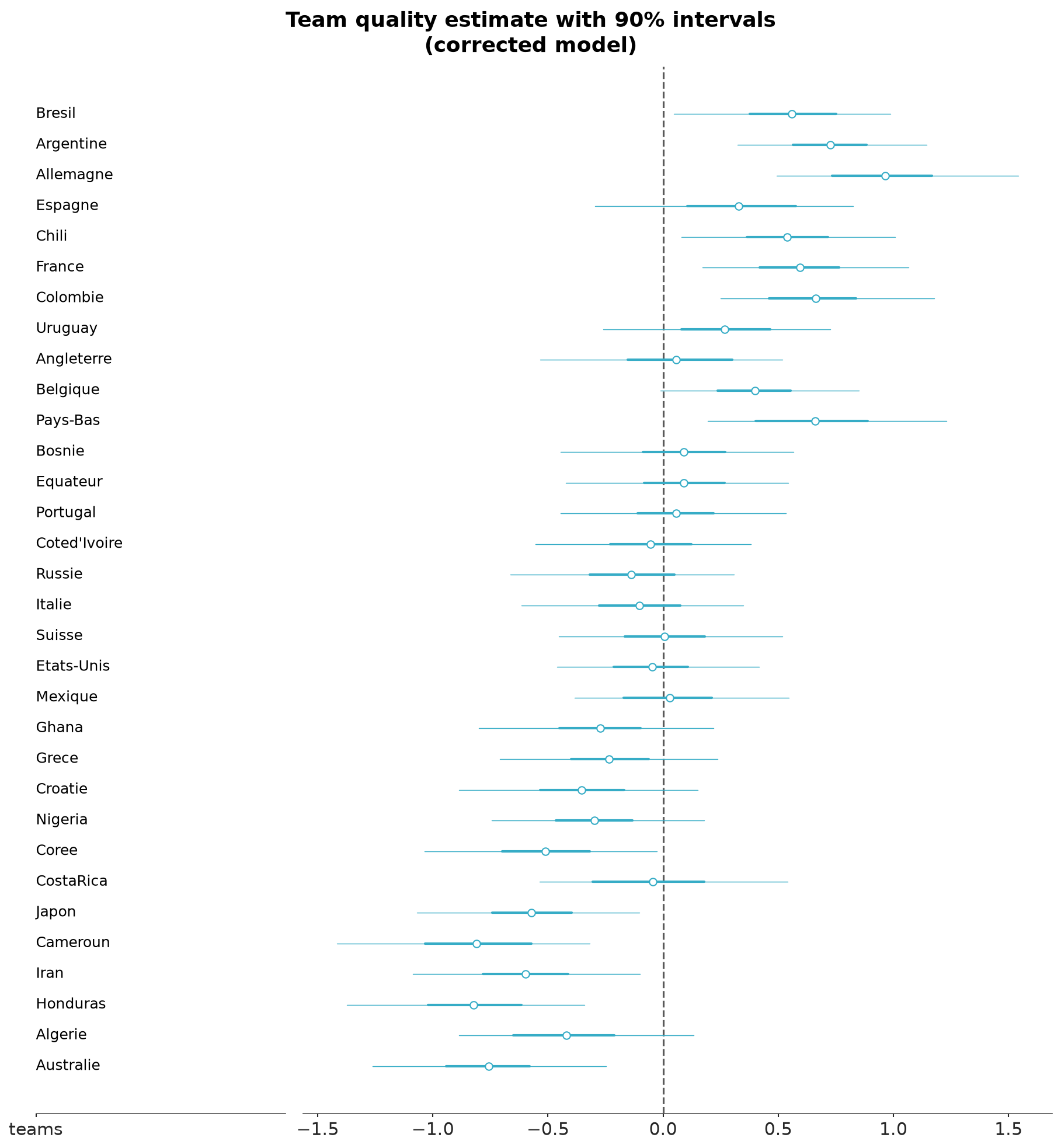
5.1 Check the fit of the fixed first model
y_rep_orig_3 = idata_3.posterior["y_rep"].values * np.abs(idata_3.posterior["y_rep"].values)
idata_3_ppc = az.from_dict({
    "posterior_predictive": {"dif": y_rep_orig_3},
    "observed_data": {"dif": dif}},
    coords={"games": gamenames},
    dims={"dif": ["games"]},
)

pc = az.plot_forest(
    idata_3_ppc,
    group="posterior_predictive",
    combined=True,
    visuals={"trunk": False},
    labels=["games"]
)

pc.map(
    az.visuals.scatter_x,
    "observations",
    data=idata_3_ppc.observed_data.ds,
    coords={"column": "forest"},
    color="C1",
)
pc.add_title("Game score differentials\ncompared to 90% predictive interval\n(corrected model with square root)")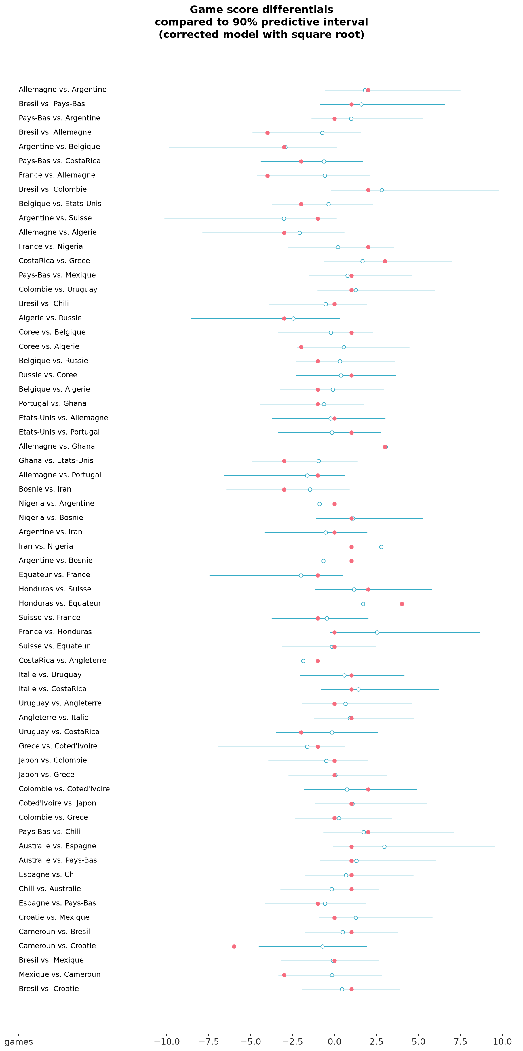
5.2 Fit the same model without the powerindex prior
Set b=0 in the data.
model_3_no_prior = CmdStanModel(stan_file="worldcup_no_prior.stan")
print_stan(model_3_no_prior)
data {
int N_teams;
int N_games;
vector[N_teams] prior_score;
array[N_games] int team_1;
array[N_games] int team_2;
vector[N_games] score_1;
vector[N_games] score_2;
real df;
real b; // To remove the prior score in the model, just set b=0 when running this program.
}
transformed data {
vector[N_games] dif = score_1 - score_2;
vector[N_games] sqrt_dif;
for (i in 1:N_games){
sqrt_dif[i] = 2 * (step(dif[i]) - 0.5) * sqrt(abs(dif[i]));
}
}
parameters {
vector[N_teams] alpha;
real<lower=0> sigma_a;
real<lower=0> sigma_y;
}
transformed parameters {
vector[N_teams] a = b * prior_score + sigma_a * alpha;
}
model {
alpha ~ normal(0, 1);
sigma_a ~ normal(0, 1);
sigma_y ~ normal(0, 1);
sqrt_dif ~ student_t(df, a[team_1] - a[team_2], sigma_y);
}
generated quantities {
vector[N_games] log_lik;
for (n in 1:N_games) {
log_lik[n] = student_t_lpdf(sqrt_dif[n] | df, a[team_1[n]] - a[team_2[n]], sigma_y);
}
}stan_data_no_prior = {**stan_data, "b": 0}
fit_3_no_prior = model_3_no_prior.sample(data=stan_data_no_prior, seed=SEED, show_progress=False)idata_3_np = az.from_cmdstanpy(
fit_3_no_prior,
observed_data={"sqrt_dif": sqrt_dif_fixed.ravel()},
log_likelihood={"sqrt_dif": "log_lik"},
coords={"a_dim_0": teamnames},
)
idata_3_np.posterior.ds = idata_3_np.posterior.ds.rename({
"a_dim_0": "teams",
})
pc = az.plot_forest(idata_3_np, var_names=["a"], combined=True, labels=["teams"])
pc.add_title("Team quality estimate with 90% intervals\nModel without prior rankings")
pc.coords = {"column": "forest"}
az.add_lines(pc, values=0)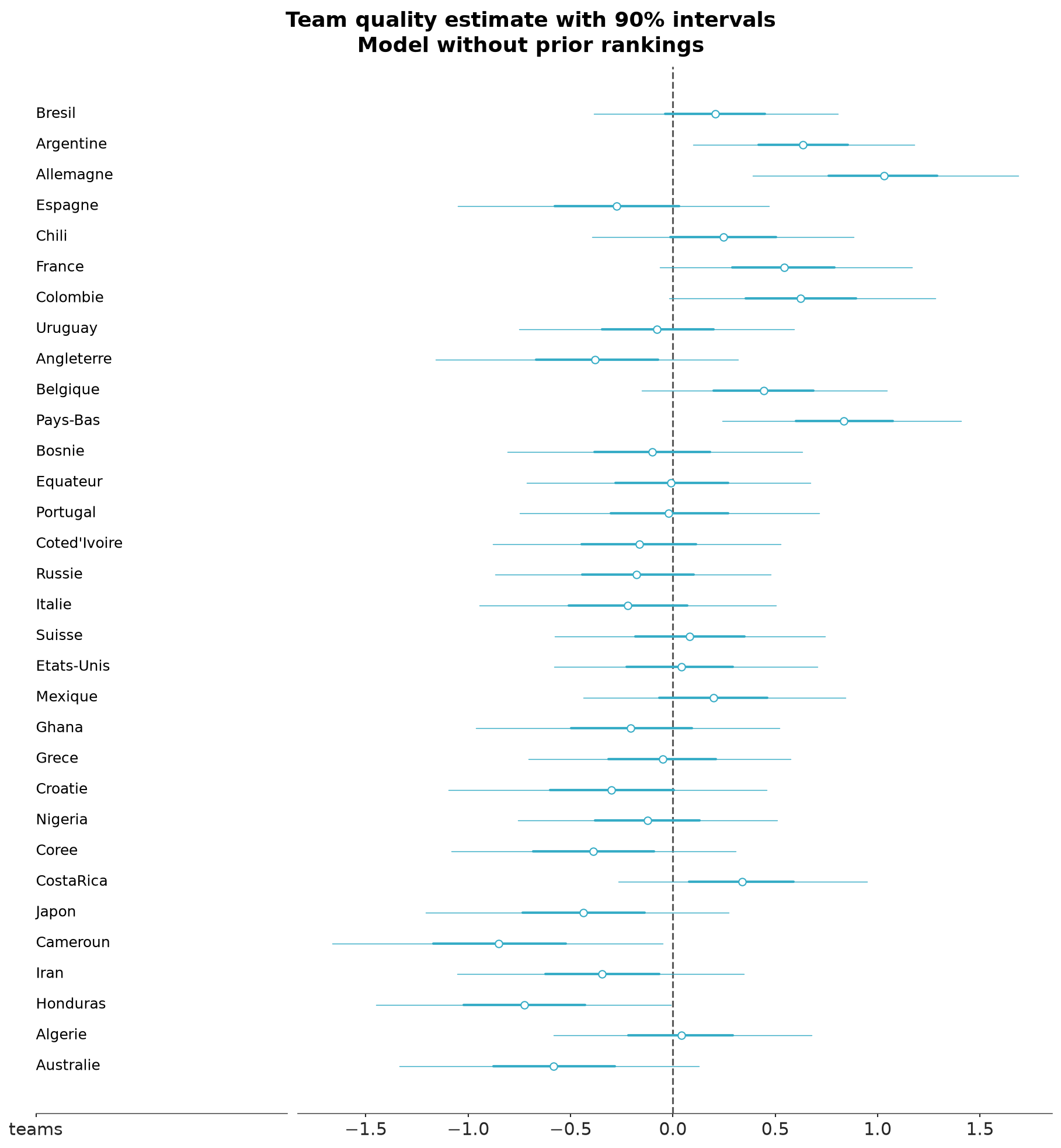
6 Discrete models and LOO-CV comparison
6.1 Discrete model with explicit latent z sampled
model_discr_z = CmdStanModel(stan_file="worldcup_discrete_z.stan")
print_stan(model_discr_z)
data {
int N_teams;
int N_games;
vector[N_teams] prior_score;
array[N_games] int team_1;
array[N_games] int team_2;
vector[N_games] score_1;
vector[N_games] score_2;
real df;
}
transformed data {
vector[N_games] dif = score_1 - score_2;
}
parameters {
vector[N_teams] alpha;
real b;
real<lower=0> sigma_a;
real<lower=0> sigma_z;
vector<lower=dif-0.5, upper=dif+0.5>[N_games] z;
}
transformed parameters {
vector[N_teams] a = b * prior_score + sigma_a * alpha;
}
model {
alpha ~ normal(0, 1);
b ~ normal(0, 1);
sigma_a ~ normal(0, 1);
sigma_z ~ normal(0, 1);
z ~ normal(a[team_1] - a[team_2], sigma_z);
}
generated quantities {
vector[N_games] y_rep;
vector[N_games] z_rep;
vector[N_games] log_lik;
for (n in 1:N_games) {
z_rep[n] = normal_rng(a[team_1[n]] - a[team_2[n]], sigma_z);
y_rep[n] = round(z_rep[n]);
log_lik[n] = log_diff_exp(normal_lcdf(dif[n]+0.5 | a[team_1[n]] - a[team_2[n]], sigma_z), normal_lcdf(dif[n]-0.5 | a[team_1[n]] - a[team_2[n]], sigma_z));
}
}fit_discr_z = model_discr_z.sample(data=stan_data, seed=SEED, show_progress=False)idata_discr_z = az.from_cmdstanpy(
fit_discr_z,
posterior_predictive="y_rep",
observed_data={"dif": dif},
log_likelihood={"dif": "log_lik"},
coords={"a_dim_0": teamnames},
)
idata_discr_z.posterior_predictive.ds = idata_discr_z.posterior_predictive.ds.rename({"y_rep": "dif", "y_rep_dim_0":"dif_dim_0"})
az.summary(idata_discr_z, var_names=["b", "sigma_a", "sigma_z"])| mean | sd | eti90_lb | eti90_ub | ess_bulk | ess_tail | r_hat | mcse_mean | mcse_sd | |
|---|---|---|---|---|---|---|---|---|---|
| b | 1.07 | 0.318 | 0.56 | 1.6 | 3570 | 2976 | 1.00 | 0.0053 | 0.0038 |
| sigma_a | 0.51 | 0.23 | 0.11 | 0.87 | 672 | 789 | 1.01 | 0.0086 | 0.0059 |
| sigma_z | 1.494 | 0.168 | 1.2 | 1.8 | 1627 | 2145 | 1.00 | 0.0042 | 0.0032 |
6.2 Discrete model with latent z integrated out
model_discr = CmdStanModel(stan_file="worldcup_discrete.stan")
print_stan(model_discr)
data {
int N_teams;
int N_games;
vector[N_teams] prior_score;
array[N_games] int team_1;
array[N_games] int team_2;
vector[N_games] score_1;
vector[N_games] score_2;
}
transformed data {
vector[N_games] dif = score_1 - score_2;
}
parameters {
vector[N_teams] alpha;
real b;
real<lower=0> sigma_a;
real<lower=0> sigma_z;
}
transformed parameters {
vector[N_teams] a = b * prior_score + sigma_a * alpha;
}
model {
alpha ~ normal(0, 1);
b ~ normal(0, 1);
sigma_a ~ normal(0, 1);
sigma_z ~ normal(0, 1);
for (n in 1:N_games) {
target += log_diff_exp(normal_lcdf(dif[n]+0.5 | a[team_1[n]] - a[team_2[n]], sigma_z),
normal_lcdf(dif[n]-0.5 | a[team_1[n]] - a[team_2[n]], sigma_z));
}
}
generated quantities {
vector[N_games] y_rep;
vector[N_games] z_rep;
vector[N_games] log_lik;
for (n in 1:N_games) {
z_rep[n] = normal_rng(a[team_1[n]] - a[team_2[n]], sigma_z);
y_rep[n] = round(z_rep[n]);
log_lik[n] = log_diff_exp(normal_lcdf(dif[n]+0.5 | a[team_1[n]] - a[team_2[n]], sigma_z), normal_lcdf(dif[n]-0.5 | a[team_1[n]] - a[team_2[n]], sigma_z));
}
}fit_discr = model_discr.sample(data=stan_data, seed=SEED, show_progress=False)idata_discr = az.from_cmdstanpy(
fit_discr,
posterior_predictive="y_rep",
observed_data={"dif": dif},
log_likelihood={"dif": "log_lik"},
coords={"a_dim_0": teamnames},
)
idata_discr.posterior_predictive.ds = idata_discr.posterior_predictive.ds.rename({"y_rep": "dif", "y_rep_dim_0":"dif_dim_0"})
az.summary(idata_discr, var_names=["a", "b", "sigma_a", "sigma_z"])| mean | sd | eti90_lb | eti90_ub | ess_bulk | ess_tail | r_hat | mcse_mean | mcse_sd | |
|---|---|---|---|---|---|---|---|---|---|
| a[Bresil] | 0.49 | 0.45 | -0.29 | 1.2 | 2869 | 2740 | 1.00 | 0.0085 | 0.0061 |
| a[Argentine] | 0.86 | 0.401 | 0.2 | 1.5 | 5577 | 3263 | 1.00 | 0.0054 | 0.004 |
| a[Allemagne] | 1.39 | 0.51 | 0.62 | 2.3 | 2213 | 2536 | 1.00 | 0.011 | 0.0075 |
| a[Espagne] | 0.33 | 0.52 | -0.63 | 1.1 | 2644 | 3048 | 1.00 | 0.01 | 0.0081 |
| a[Chili] | 0.65 | 0.447 | -0.11 | 1.4 | 5658 | 3433 | 1.00 | 0.0059 | 0.0046 |
| a[France] | 0.92 | 0.45 | 0.24 | 1.7 | 3673 | 3104 | 1.00 | 0.0074 | 0.0056 |
| a[Colombie] | 0.87 | 0.47 | 0.19 | 1.7 | 4038 | 3007 | 1.00 | 0.0073 | 0.0059 |
| a[Uruguay] | 0.26 | 0.46 | -0.52 | 0.95 | 4215 | 2933 | 1.00 | 0.0071 | 0.0057 |
| a[Angleterre] | 0.16 | 0.48 | -0.72 | 0.87 | 3980 | 2979 | 1.00 | 0.0078 | 0.006 |
| a[Belgique] | 0.43 | 0.409 | -0.23 | 1.1 | 5599 | 3100 | 1.01 | 0.0055 | 0.0047 |
| a[Pays-Bas] | 0.92 | 0.48 | 0.22 | 1.8 | 2152 | 2339 | 1.00 | 0.01 | 0.0071 |
| a[Bosnie] | 0.18 | 0.454 | -0.59 | 0.92 | 6516 | 3028 | 1.00 | 0.0057 | 0.0049 |
| a[Equateur] | 0.13 | 0.46 | -0.66 | 0.86 | 5844 | 3358 | 1.00 | 0.006 | 0.0053 |
| a[Portugal] | -0.05 | 0.45 | -0.84 | 0.64 | 4538 | 3283 | 1.00 | 0.0069 | 0.0059 |
| a[Coted'Ivoire] | -0.04 | 0.46 | -0.84 | 0.68 | 5785 | 2967 | 1.00 | 0.0061 | 0.0054 |
| a[Russie] | -0.12 | 0.46 | -0.93 | 0.61 | 4776 | 3092 | 1.00 | 0.0067 | 0.0056 |
| a[Italie] | -0.08 | 0.459 | -0.85 | 0.67 | 6509 | 2903 | 1.00 | 0.0057 | 0.0047 |
| a[Suisse] | 0.01 | 0.43 | -0.67 | 0.73 | 5125 | 3139 | 1.00 | 0.006 | 0.005 |
| a[Etats-Unis] | -0.05 | 0.44 | -0.73 | 0.71 | 5757 | 3016 | 1.00 | 0.0059 | 0.0049 |
| a[Mexique] | -0.01 | 0.44 | -0.69 | 0.77 | 5104 | 3553 | 1.00 | 0.0062 | 0.005 |
| a[Ghana] | -0.25 | 0.45 | -0.99 | 0.51 | 5217 | 2577 | 1.00 | 0.0063 | 0.0055 |
| a[Grece] | -0.36 | 0.42 | -1 | 0.33 | 5400 | 3301 | 1.00 | 0.0058 | 0.0052 |
| a[Croatie] | -0.36 | 0.46 | -1.1 | 0.39 | 5982 | 2374 | 1.00 | 0.006 | 0.005 |
| a[Nigeria] | -0.35 | 0.44 | -1 | 0.41 | 4995 | 3366 | 1.00 | 0.0063 | 0.0054 |
| a[Coree] | -0.63 | 0.48 | -1.4 | 0.12 | 5668 | 3209 | 1.00 | 0.0063 | 0.0054 |
| a[CostaRica] | -0.07 | 0.5 | -0.78 | 0.83 | 2711 | 3209 | 1.00 | 0.0096 | 0.007 |
| a[Japon] | -0.75 | 0.47 | -1.5 | -0.013 | 5479 | 3501 | 1.00 | 0.0064 | 0.0052 |
| a[Cameroun] | -1.19 | 0.58 | -2.3 | -0.38 | 2350 | 2972 | 1.00 | 0.012 | 0.0096 |
| a[Iran] | -0.74 | 0.49 | -1.6 | 0.064 | 6082 | 3306 | 1.00 | 0.0063 | 0.0054 |
| a[Honduras] | -1.08 | 0.51 | -2 | -0.34 | 3761 | 3277 | 1.00 | 0.0083 | 0.0068 |
| a[Algerie] | -0.48 | 0.51 | -1.2 | 0.44 | 2995 | 3065 | 1.00 | 0.0093 | 0.0072 |
| a[Australie] | -1.01 | 0.48 | -1.8 | -0.29 | 5184 | 3235 | 1.00 | 0.0066 | 0.0055 |
| b | 1.08 | 0.314 | 0.56 | 1.6 | 3803 | 2989 | 1.00 | 0.0051 | 0.004 |
| sigma_a | 0.51 | 0.219 | 0.13 | 0.87 | 1078 | 1113 | 1.00 | 0.0066 | 0.0045 |
| sigma_z | 1.494 | 0.165 | 1.2 | 1.8 | 2069 | 2514 | 1.00 | 0.0036 | 0.0027 |
6.3 Discrete model with no power score
model_discr_nopower = CmdStanModel(stan_file="worldcup_discrete_nopower.stan")
print_stan(model_discr_nopower)
data {
int N_teams;
int N_games;
array[N_games] int team_1;
array[N_games] int team_2;
vector[N_games] score_1;
vector[N_games] score_2;
}
transformed data {
vector[N_games] dif = score_1 - score_2;
}
parameters {
vector[N_teams] alpha;
real<lower=0> sigma_a;
real<lower=0> sigma_z;
}
transformed parameters {
vector[N_teams] a = sigma_a * alpha;
}
model {
alpha ~ normal(0, 1);
sigma_a ~ normal(0, 1);
sigma_z ~ normal(0, 1);
for (n in 1:N_games) {
target += log_diff_exp(normal_lcdf(dif[n]+0.5 | a[team_1[n]] - a[team_2[n]], sigma_z),
normal_lcdf(dif[n]-0.5 | a[team_1[n]] - a[team_2[n]], sigma_z));
}
}
generated quantities {
vector[N_games] y_rep;
vector[N_games] z_rep;
vector[N_games] log_lik;
for (n in 1:N_games) {
real a_dif_n = a[team_1[n]] - a[team_2[n]];
z_rep[n] = normal_rng(a_dif_n, sigma_z);
y_rep[n] = round(z_rep[n]);
log_lik[n] = log_diff_exp(normal_lcdf(dif[n]+0.5 | a_dif_n, sigma_z),
normal_lcdf(dif[n]-0.5 | a_dif_n, sigma_z));
}
}fit_discr_nopower = model_discr_nopower.sample(data=stan_data, seed=SEED, show_progress=False)idata_discr_np = az.from_cmdstanpy(
fit_discr_nopower,
posterior_predictive="y_rep",
observed_data={"dif": dif},
log_likelihood={"dif": "log_lik"},
coords={"a_dim_0": teamnames},
)
idata_discr_np.posterior_predictive.ds = idata_discr_np.posterior_predictive.ds.rename({"y_rep": "dif", "y_rep_dim_0":"dif_dim_0"})
az.summary(idata_discr_np, var_names=["a", "sigma_a", "sigma_z"])| mean | sd | eti90_lb | eti90_ub | ess_bulk | ess_tail | r_hat | mcse_mean | mcse_sd | |
|---|---|---|---|---|---|---|---|---|---|
| a[Bresil] | -0.06 | 0.467 | -0.83 | 0.72 | 5670 | 3322 | 1.00 | 0.0062 | 0.0048 |
| a[Argentine] | 0.55 | 0.52 | -0.25 | 1.4 | 2360 | 2841 | 1.00 | 0.011 | 0.0075 |
| a[Allemagne] | 1.3 | 0.66 | 0.14 | 2.4 | 1105 | 856 | 1.00 | 0.02 | 0.013 |
| a[Espagne] | -0.34 | 0.6 | -1.4 | 0.57 | 4192 | 3088 | 1.00 | 0.0091 | 0.0073 |
| a[Chili] | 0.22 | 0.56 | -0.67 | 1.2 | 5149 | 3479 | 1.00 | 0.0079 | 0.0061 |
| a[France] | 0.8 | 0.59 | -0.11 | 1.8 | 2037 | 1614 | 1.00 | 0.013 | 0.009 |
| a[Colombie] | 0.71 | 0.57 | -0.15 | 1.7 | 2480 | 2284 | 1.00 | 0.011 | 0.0077 |
| a[Uruguay] | -0.16 | 0.56 | -1.1 | 0.76 | 6099 | 3270 | 1.00 | 0.0072 | 0.0055 |
| a[Angleterre] | -0.27 | 0.6 | -1.3 | 0.67 | 5134 | 2963 | 1.00 | 0.0085 | 0.0068 |
| a[Belgique] | 0.36 | 0.53 | -0.49 | 1.3 | 4207 | 3441 | 1.00 | 0.0082 | 0.0059 |
| a[Pays-Bas] | 0.95 | 0.57 | 0.015 | 1.9 | 1611 | 1186 | 1.00 | 0.014 | 0.0096 |
| a[Bosnie] | 0.04 | 0.59 | -0.94 | 0.97 | 5795 | 3008 | 1.00 | 0.0076 | 0.0062 |
| a[Equateur] | 0.02 | 0.58 | -0.92 | 0.98 | 6613 | 3476 | 1.00 | 0.0071 | 0.0058 |
| a[Portugal] | -0.21 | 0.59 | -1.2 | 0.75 | 6091 | 3137 | 1.00 | 0.0076 | 0.006 |
| a[Coted'Ivoire] | -0.13 | 0.6 | -1.1 | 0.83 | 5892 | 3058 | 1.00 | 0.0078 | 0.0062 |
| a[Russie] | -0.1 | 0.6 | -1.1 | 0.89 | 6636 | 3276 | 1.00 | 0.0073 | 0.0058 |
| a[Italie] | -0.15 | 0.59 | -1.2 | 0.79 | 5814 | 3286 | 1.00 | 0.0077 | 0.0058 |
| a[Suisse] | 0.07 | 0.56 | -0.85 | 1 | 5616 | 2678 | 1.00 | 0.0075 | 0.0056 |
| a[Etats-Unis] | 0.06 | 0.56 | -0.85 | 0.98 | 4723 | 2841 | 1.00 | 0.0082 | 0.0065 |
| a[Mexique] | 0.18 | 0.55 | -0.73 | 1.1 | 5899 | 2919 | 1.00 | 0.0072 | 0.0056 |
| a[Ghana] | -0.09 | 0.59 | -1.1 | 0.86 | 6482 | 2981 | 1.00 | 0.0074 | 0.0057 |
| a[Grece] | -0.18 | 0.55 | -1.1 | 0.66 | 5382 | 3324 | 1.00 | 0.0076 | 0.006 |
| a[Croatie] | -0.16 | 0.59 | -1.2 | 0.78 | 4432 | 2730 | 1.00 | 0.009 | 0.0071 |
| a[Nigeria] | -0.09 | 0.57 | -1 | 0.83 | 6042 | 3278 | 1.00 | 0.0074 | 0.0059 |
| a[Coree] | -0.33 | 0.59 | -1.3 | 0.59 | 4804 | 3303 | 1.00 | 0.0085 | 0.0066 |
| a[CostaRica] | 0.33 | 0.53 | -0.51 | 1.2 | 4758 | 3421 | 1.00 | 0.0077 | 0.0056 |
| a[Japon] | -0.49 | 0.62 | -1.5 | 0.48 | 3492 | 2770 | 1.00 | 0.01 | 0.008 |
| a[Cameroun] | -1.11 | 0.75 | -2.4 | 0.02 | 1348 | 1097 | 1.00 | 0.02 | 0.014 |
| a[Iran] | -0.32 | 0.6 | -1.4 | 0.63 | 4489 | 2979 | 1.00 | 0.0089 | 0.0072 |
| a[Honduras] | -0.83 | 0.66 | -2 | 0.15 | 2201 | 1901 | 1.00 | 0.014 | 0.01 |
| a[Algerie] | 0.17 | 0.56 | -0.7 | 1.1 | 5450 | 3288 | 1.00 | 0.0075 | 0.0061 |
| a[Australie] | -0.7 | 0.65 | -1.8 | 0.25 | 2421 | 3022 | 1.00 | 0.013 | 0.0099 |
| sigma_a | 0.75 | 0.24 | 0.33 | 1.1 | 721 | 795 | 1.00 | 0.0095 | 0.0078 |
| sigma_z | 1.52 | 0.19 | 1.2 | 1.9 | 1270 | 1353 | 1.00 | 0.0055 | 0.0041 |
6.4 Discrete model with power score only
model_discr_poweronly = CmdStanModel(stan_file="worldcup_discrete_poweronly.stan")
print_stan(model_discr_poweronly)
data {
int N_teams;
int N_games;
vector[N_teams] prior_score;
array[N_games] int team_1;
array[N_games] int team_2;
vector[N_games] score_1;
vector[N_games] score_2;
}
transformed data {
vector[N_games] dif = score_1 - score_2;
}
parameters {
real b0;
real b;
real<lower=0> sigma_z;
}
transformed parameters {
vector[N_teams] a = b0 + b * prior_score;
}
model {
b0 ~ normal(0, 1);
b ~ normal(0, 1);
sigma_z ~ normal(0, 1);
for (n in 1:N_games) {
target += log_diff_exp(normal_lcdf(dif[n]+0.5 | a[team_1[n]] - a[team_2[n]], sigma_z),
normal_lcdf(dif[n]-0.5 | a[team_1[n]] - a[team_2[n]], sigma_z));
}
}
generated quantities {
vector[N_games] y_rep;
vector[N_games] z_rep;
vector[N_games] log_lik;
for (n in 1:N_games) {
z_rep[n] = normal_rng(a[team_1[n]] - a[team_2[n]], sigma_z);
y_rep[n] = round(z_rep[n]);
log_lik[n] = log_diff_exp(normal_lcdf(dif[n]+0.5 | a[team_1[n]] - a[team_2[n]], sigma_z), normal_lcdf(dif[n]-0.5 | a[team_1[n]] - a[team_2[n]], sigma_z));
}
}fit_discr_poweronly = model_discr_poweronly.sample(data=stan_data, seed=SEED, show_progress=False)idata_discr_po = az.from_cmdstanpy(
fit_discr_poweronly,
posterior_predictive="y_rep",
observed_data={"dif": dif},
log_likelihood={"dif": "log_lik"},
coords={"a_dim_0": teamnames},
)
idata_discr_po.posterior_predictive.ds = idata_discr_po.posterior_predictive.ds.rename({"y_rep": "dif", "y_rep_dim_0":"dif_dim_0"})
az.summary(idata_discr_po, var_names=["b0", "b", "sigma_z"])| mean | sd | eti90_lb | eti90_ub | ess_bulk | ess_tail | r_hat | mcse_mean | mcse_sd | |
|---|---|---|---|---|---|---|---|---|---|
| b0 | 0 | 1.02 | -1.7 | 1.7 | 3564 | 2463 | 1.00 | 0.017 | 0.012 |
| b | 1.069 | 0.275 | 0.61 | 1.5 | 3810 | 2831 | 1.00 | 0.0045 | 0.0032 |
| sigma_z | 1.649 | 0.148 | 1.4 | 1.9 | 3827 | 2755 | 1.00 | 0.0024 | 0.0018 |
6.5 Discrete model with no power score and pooled effect
model_discr_pool = CmdStanModel(stan_file="worldcup_discrete_pooled.stan")
print_stan(model_discr_pool)
data {
int N_teams;
int N_games;
vector[N_teams] prior_score;
array[N_games] int team_1;
array[N_games] int team_2;
vector[N_games] score_1;
vector[N_games] score_2;
}
transformed data {
vector[N_games] dif = score_1 - score_2;
}
parameters {
real mu_z;
real<lower=0> sigma_z;
}
model {
mu_z ~ normal(0, 1);
sigma_z ~ normal(0, 1);
for (n in 1:N_games) {
target += log_diff_exp(normal_lcdf(dif[n]+0.5 | mu_z, sigma_z),
normal_lcdf(dif[n]-0.5 | mu_z, sigma_z));
}
}
generated quantities {
vector[N_games] y_rep;
vector[N_games] z_rep;
vector[N_games] log_lik;
for (n in 1:N_games) {
z_rep[n] = normal_rng(mu_z, sigma_z);
y_rep[n] = round(z_rep[n]);
log_lik[n] = log_diff_exp(normal_lcdf(dif[n]+0.5 | mu_z, sigma_z), normal_lcdf(dif[n]-0.5 | mu_z, sigma_z));
}
}fit_discr_pool = model_discr_pool.sample(data=stan_data, seed=SEED, show_progress=False)idata_discr_pl = az.from_cmdstanpy(
fit_discr_pool,
posterior_predictive="y_rep",
observed_data={"dif": dif},
log_likelihood={"dif": "log_lik"},
coords={"a_dim_0": teamnames},
)
idata_discr_pl.posterior_predictive.ds = idata_discr_pl.posterior_predictive.ds.rename({"y_rep": "dif", "y_rep_dim_0":"dif_dim_0"})
az.summary(idata_discr_pl, var_names=["mu_z", "sigma_z"])| mean | sd | eti90_lb | eti90_ub | ess_bulk | ess_tail | r_hat | mcse_mean | mcse_sd | |
|---|---|---|---|---|---|---|---|---|---|
| mu_z | -0.124 | 0.23 | -0.49 | 0.25 | 3571 | 2704 | 1.00 | 0.0039 | 0.0028 |
| sigma_z | 1.847 | 0.166 | 1.6 | 2.1 | 3712 | 2659 | 1.00 | 0.0027 | 0.002 |
6.6 Model comparison
Now that we have implemented discrete model, we compare various models with or without different components. Hierarchical model with power score is the best, but not much better than power score only model or hierarchical model without power score. Clearly the power score and the score differences are providing similar information. Looking at the posterior we do see that using them both, does decrease posterior uncertainty, but as the match outcomes still have significant randomness the difference in predictive performance is small.
az.compare({
    "Hier. w power score": idata_discr,
    "Power score only": idata_discr_po,
    "Hier. w/o power score": idata_discr_np,
    "Pooled w/o power score": idata_discr_pl,
})
/home/osvaldo/anaconda3/envs/bwb/lib/python3.14/site-packages/arviz_stats/loo/helper_loo.py:1146: UserWarning: Estimated shape parameter of Pareto distribution is greater than 0.70 for one or more samples. You should consider using a more robust model, this is because importance sampling is less likely to work well if the marginal posterior and LOO posterior are very different. This is more likely to happen with a non-robust model and highly influential observations.
warnings.warn(| rank | elpd_diff | dse | p_worse | diag_diff | diag_elpd | p | elpd | se | weight | |
|---|---|---|---|---|---|---|---|---|---|---|
| Hier. w power score | 0 | 0.0 | 0.0 | NaN | 11.7 | -120.0 | 8.2 | 0.78 | ||
| Power score only | 1 | -1.0 | 1.7 | 0.81 | N < 100 | 2.7 | -130.0 | 9.0 | 0.11 | |
| Hier. w/o power score | 2 | -3.0 | 2.8 | 0.89 | N < 100 | 2 k̂ > 0.70 | 14.9 | -130.0 | 7.0 | 0.11 |
| Pooled w/o power score | 3 | -8.0 | 3.4 | 0.99 | N < 100 | 2.3 | -130.0 | 6.9 | 0.00 |
7 Discretizing continuous models
7.1 Continuous model with log predictive probability using midpoint rule
model_cont_midp = CmdStanModel(stan_file="worldcup_continuous_midpoint_ll.stan")
print_stan(model_cont_midp)
data {
int N_teams;
int N_games;
vector[N_teams] prior_score;
array[N_games] int team_1;
array[N_games] int team_2;
vector[N_games] score_1;
vector[N_games] score_2;
}
transformed data {
vector[N_games] dif = score_1 - score_2;
}
parameters {
vector[N_teams] alpha;
real b;
real<lower=0> sigma_a;
real<lower=0> sigma_y;
}
transformed parameters {
vector[N_teams] a = b * prior_score + sigma_a * alpha;
}
model {
alpha ~ normal(0, 1);
b ~ normal(0, 1);
sigma_a ~ normal(0, 1);
sigma_y ~ normal(0, 1);
dif ~ normal(a[team_1] - a[team_2], sigma_y);
}
generated quantities {
vector[N_games] y_rep;
vector[N_games] log_lik;
for (n in 1:N_games) {
y_rep[n] = normal_rng(a[team_1[n]] - a[team_2[n]], sigma_y);
log_lik[n] = normal_lpdf(dif[n] | a[team_1[n]] - a[team_2[n]], sigma_y);
}
}fit_cont_midp = model_cont_midp.sample(data=stan_data, seed=SEED, show_progress=False)idata_cont_mp = az.from_cmdstanpy(
fit_cont_midp,
posterior_predictive="y_rep",
observed_data={"dif": dif},
log_likelihood={"dif": "log_lik"},
coords={"a_dim_0": teamnames},
)
idata_cont_mp.posterior_predictive.ds = idata_cont_mp.posterior_predictive.ds.rename({"y_rep": "dif", "y_rep_dim_0":"dif_dim_0"})
az.summary(idata_cont_mp, var_names=["a", "b", "sigma_a", "sigma_y"])| mean | sd | eti90_lb | eti90_ub | ess_bulk | ess_tail | r_hat | mcse_mean | mcse_sd | |
|---|---|---|---|---|---|---|---|---|---|
| a[Bresil] | 0.49 | 0.44 | -0.25 | 1.1 | 2972 | 2898 | 1.00 | 0.0079 | 0.0058 |
| a[Argentine] | 0.85 | 0.412 | 0.18 | 1.5 | 5830 | 3165 | 1.00 | 0.0054 | 0.0042 |
| a[Allemagne] | 1.38 | 0.51 | 0.63 | 2.3 | 1645 | 1792 | 1.00 | 0.012 | 0.0086 |
| a[Espagne] | 0.33 | 0.53 | -0.62 | 1.1 | 3668 | 3167 | 1.00 | 0.0086 | 0.0067 |
| a[Chili] | 0.66 | 0.439 | -0.064 | 1.4 | 6553 | 2903 | 1.00 | 0.0054 | 0.0046 |
| a[France] | 0.9 | 0.46 | 0.22 | 1.7 | 3763 | 3124 | 1.00 | 0.0075 | 0.0057 |
| a[Colombie] | 0.86 | 0.45 | 0.19 | 1.7 | 3802 | 2753 | 1.00 | 0.0072 | 0.0058 |
| a[Uruguay] | 0.24 | 0.47 | -0.59 | 0.95 | 4422 | 3086 | 1.00 | 0.007 | 0.0059 |
| a[Angleterre] | 0.14 | 0.5 | -0.75 | 0.87 | 4490 | 2835 | 1.00 | 0.0077 | 0.0064 |
| a[Belgique] | 0.43 | 0.421 | -0.24 | 1.1 | 6592 | 3326 | 1.00 | 0.0052 | 0.0045 |
| a[Pays-Bas] | 0.92 | 0.48 | 0.22 | 1.8 | 1648 | 1994 | 1.00 | 0.012 | 0.0082 |
| a[Bosnie] | 0.17 | 0.444 | -0.59 | 0.9 | 6526 | 3496 | 1.00 | 0.0056 | 0.0047 |
| a[Equateur] | 0.14 | 0.45 | -0.63 | 0.86 | 8081 | 3003 | 1.00 | 0.0051 | 0.0043 |
| a[Portugal] | -0.03 | 0.45 | -0.81 | 0.65 | 5579 | 3090 | 1.00 | 0.006 | 0.0052 |
| a[Coted'Ivoire] | -0.04 | 0.44 | -0.81 | 0.65 | 4517 | 3085 | 1.00 | 0.0065 | 0.0057 |
| a[Russie] | -0.11 | 0.47 | -0.93 | 0.64 | 5423 | 3158 | 1.00 | 0.0063 | 0.0053 |
| a[Italie] | -0.09 | 0.44 | -0.85 | 0.61 | 5963 | 3171 | 1.00 | 0.0058 | 0.0054 |
| a[Suisse] | -0.01 | 0.434 | -0.71 | 0.74 | 6035 | 3499 | 1.00 | 0.0056 | 0.0046 |
| a[Etats-Unis] | -0.04 | 0.42 | -0.69 | 0.68 | 5132 | 3192 | 1.00 | 0.0059 | 0.0052 |
| a[Mexique] | -0 | 0.45 | -0.72 | 0.81 | 5038 | 3315 | 1.00 | 0.0064 | 0.0052 |
| a[Ghana] | -0.23 | 0.45 | -0.95 | 0.55 | 6544 | 3434 | 1.00 | 0.0057 | 0.0048 |
| a[Grece] | -0.37 | 0.431 | -1.1 | 0.34 | 6882 | 2994 | 1.00 | 0.0052 | 0.0043 |
| a[Croatie] | -0.35 | 0.46 | -1.1 | 0.42 | 6205 | 3036 | 1.00 | 0.0059 | 0.0052 |
| a[Nigeria] | -0.35 | 0.433 | -1 | 0.38 | 6538 | 3231 | 1.00 | 0.0054 | 0.0043 |
| a[Coree] | -0.62 | 0.471 | -1.4 | 0.12 | 6526 | 3365 | 1.00 | 0.0059 | 0.0049 |
| a[CostaRica] | -0.09 | 0.47 | -0.77 | 0.75 | 2570 | 2880 | 1.00 | 0.0093 | 0.0065 |
| a[Japon] | -0.74 | 0.46 | -1.5 | -0.018 | 6356 | 3109 | 1.00 | 0.0059 | 0.005 |
| a[Cameroun] | -1.17 | 0.57 | -2.2 | -0.37 | 2368 | 3213 | 1.00 | 0.011 | 0.0089 |
| a[Iran] | -0.73 | 0.472 | -1.5 | 0.039 | 6350 | 2791 | 1.00 | 0.006 | 0.0049 |
| a[Honduras] | -1.07 | 0.49 | -1.9 | -0.35 | 4262 | 3411 | 1.00 | 0.0076 | 0.0064 |
| a[Algerie] | -0.47 | 0.5 | -1.2 | 0.42 | 3115 | 3487 | 1.00 | 0.0089 | 0.0068 |
| a[Australie] | -1 | 0.49 | -1.8 | -0.23 | 5606 | 3175 | 1.00 | 0.0065 | 0.0056 |
| b | 1.073 | 0.307 | 0.56 | 1.6 | 4393 | 2710 | 1.00 | 0.0047 | 0.0034 |
| sigma_a | 0.5 | 0.219 | 0.11 | 0.85 | 898 | 1120 | 1.00 | 0.0072 | 0.0049 |
| sigma_y | 1.52 | 0.164 | 1.3 | 1.8 | 2030 | 2823 | 1.00 | 0.0036 | 0.0028 |
7.2 Continuous model with log predictive probability using exact integration
model_cont = CmdStanModel(stan_file="worldcup_continuous.stan")
print_stan(model_cont)
data {
int N_teams;
int N_games;
vector[N_teams] prior_score;
array[N_games] int team_1;
array[N_games] int team_2;
vector[N_games] score_1;
vector[N_games] score_2;
}
transformed data {
vector[N_games] dif = score_1 - score_2;
}
parameters {
vector[N_teams] alpha; // latent team abilities
real b; // prior weight
real<lower=0> sigma_a; // scale of ability prior distribution
real<lower=0> sigma_y; // scale of score difference distribution
}
transformed parameters {
// team abilities as weighted sum of prior score and latent team ability
vector[N_teams] a = b * prior_score + sigma_a * alpha;
}
model {
alpha ~ normal(0, 1);
b ~ normal(0, 1);
sigma_a ~ normal(0, 1);
sigma_y ~ normal(0, 1);
dif ~ normal(a[team_1] - a[team_2], sigma_y);
}
generated quantities {
vector[N_games] y_rep;
vector[N_games] log_lik;
for (n in 1:N_games) {
y_rep[n] = normal_rng(a[team_1[n]] - a[team_2[n]], sigma_y);
log_lik[n] = log_diff_exp(normal_lcdf(dif[n]+0.5 | a[team_1[n]] - a[team_2[n]], sigma_y), normal_lcdf(dif[n]-0.5 | a[team_1[n]] - a[team_2[n]], sigma_y));
}
}fit_cont = model_cont.sample(data=stan_data, seed=SEED, show_progress=False)idata_cont = az.from_cmdstanpy(
fit_cont,
posterior_predictive="y_rep",
observed_data={"dif": dif},
log_likelihood={"dif": "log_lik"},
coords={"a_dim_0": teamnames},
)
idata_cont.posterior_predictive.ds = idata_cont.posterior_predictive.ds.rename({"y_rep": "dif", "y_rep_dim_0":"dif_dim_0"})
az.summary(idata_cont, var_names=["a", "b", "sigma_a", "sigma_y"])| mean | sd | eti90_lb | eti90_ub | ess_bulk | ess_tail | r_hat | mcse_mean | mcse_sd | |
|---|---|---|---|---|---|---|---|---|---|
| a[Bresil] | 0.49 | 0.44 | -0.25 | 1.1 | 2972 | 2898 | 1.00 | 0.0079 | 0.0058 |
| a[Argentine] | 0.85 | 0.412 | 0.18 | 1.5 | 5830 | 3165 | 1.00 | 0.0054 | 0.0042 |
| a[Allemagne] | 1.38 | 0.51 | 0.63 | 2.3 | 1645 | 1792 | 1.00 | 0.012 | 0.0086 |
| a[Espagne] | 0.33 | 0.53 | -0.62 | 1.1 | 3668 | 3167 | 1.00 | 0.0086 | 0.0067 |
| a[Chili] | 0.66 | 0.439 | -0.064 | 1.4 | 6553 | 2903 | 1.00 | 0.0054 | 0.0046 |
| a[France] | 0.9 | 0.46 | 0.22 | 1.7 | 3763 | 3124 | 1.00 | 0.0075 | 0.0057 |
| a[Colombie] | 0.86 | 0.45 | 0.19 | 1.7 | 3802 | 2753 | 1.00 | 0.0072 | 0.0058 |
| a[Uruguay] | 0.24 | 0.47 | -0.59 | 0.95 | 4422 | 3086 | 1.00 | 0.007 | 0.0059 |
| a[Angleterre] | 0.14 | 0.5 | -0.75 | 0.87 | 4490 | 2835 | 1.00 | 0.0077 | 0.0064 |
| a[Belgique] | 0.43 | 0.421 | -0.24 | 1.1 | 6592 | 3326 | 1.00 | 0.0052 | 0.0045 |
| a[Pays-Bas] | 0.92 | 0.48 | 0.22 | 1.8 | 1648 | 1994 | 1.00 | 0.012 | 0.0082 |
| a[Bosnie] | 0.17 | 0.444 | -0.59 | 0.9 | 6526 | 3496 | 1.00 | 0.0056 | 0.0047 |
| a[Equateur] | 0.14 | 0.45 | -0.63 | 0.86 | 8081 | 3003 | 1.00 | 0.0051 | 0.0043 |
| a[Portugal] | -0.03 | 0.45 | -0.81 | 0.65 | 5579 | 3090 | 1.00 | 0.006 | 0.0052 |
| a[Coted'Ivoire] | -0.04 | 0.44 | -0.81 | 0.65 | 4517 | 3085 | 1.00 | 0.0065 | 0.0057 |
| a[Russie] | -0.11 | 0.47 | -0.93 | 0.64 | 5423 | 3158 | 1.00 | 0.0063 | 0.0053 |
| a[Italie] | -0.09 | 0.44 | -0.85 | 0.61 | 5963 | 3171 | 1.00 | 0.0058 | 0.0054 |
| a[Suisse] | -0.01 | 0.434 | -0.71 | 0.74 | 6035 | 3499 | 1.00 | 0.0056 | 0.0046 |
| a[Etats-Unis] | -0.04 | 0.42 | -0.69 | 0.68 | 5132 | 3192 | 1.00 | 0.0059 | 0.0052 |
| a[Mexique] | -0 | 0.45 | -0.72 | 0.81 | 5038 | 3315 | 1.00 | 0.0064 | 0.0052 |
| a[Ghana] | -0.23 | 0.45 | -0.95 | 0.55 | 6544 | 3434 | 1.00 | 0.0057 | 0.0048 |
| a[Grece] | -0.37 | 0.431 | -1.1 | 0.34 | 6882 | 2994 | 1.00 | 0.0052 | 0.0043 |
| a[Croatie] | -0.35 | 0.46 | -1.1 | 0.42 | 6205 | 3036 | 1.00 | 0.0059 | 0.0052 |
| a[Nigeria] | -0.35 | 0.433 | -1 | 0.38 | 6538 | 3231 | 1.00 | 0.0054 | 0.0043 |
| a[Coree] | -0.62 | 0.471 | -1.4 | 0.12 | 6526 | 3365 | 1.00 | 0.0059 | 0.0049 |
| a[CostaRica] | -0.09 | 0.47 | -0.77 | 0.75 | 2570 | 2880 | 1.00 | 0.0093 | 0.0065 |
| a[Japon] | -0.74 | 0.46 | -1.5 | -0.018 | 6356 | 3109 | 1.00 | 0.0059 | 0.005 |
| a[Cameroun] | -1.17 | 0.57 | -2.2 | -0.37 | 2368 | 3213 | 1.00 | 0.011 | 0.0089 |
| a[Iran] | -0.73 | 0.472 | -1.5 | 0.039 | 6350 | 2791 | 1.00 | 0.006 | 0.0049 |
| a[Honduras] | -1.07 | 0.49 | -1.9 | -0.35 | 4262 | 3411 | 1.00 | 0.0076 | 0.0064 |
| a[Algerie] | -0.47 | 0.5 | -1.2 | 0.42 | 3115 | 3487 | 1.00 | 0.0089 | 0.0068 |
| a[Australie] | -1 | 0.49 | -1.8 | -0.23 | 5606 | 3175 | 1.00 | 0.0065 | 0.0056 |
| b | 1.073 | 0.307 | 0.56 | 1.6 | 4393 | 2710 | 1.00 | 0.0047 | 0.0034 |
| sigma_a | 0.5 | 0.219 | 0.11 | 0.85 | 898 | 1120 | 1.00 | 0.0072 | 0.0049 |
| sigma_y | 1.52 | 0.164 | 1.3 | 1.8 | 2030 | 2823 | 1.00 | 0.0036 | 0.0028 |
7.3 Model comparison
The elpd_diff’s between models are small enough to be caused by Monte Carlo variation.
az.compare({
    "Discrete model": idata_discr,
    "Continuous + midpoint log_lik": idata_cont_mp,
    "Continuous model": idata_cont,
})
/home/osvaldo/anaconda3/envs/bwb/lib/python3.14/site-packages/arviz_stats/loo/helper_loo.py:1146: UserWarning: Estimated shape parameter of Pareto distribution is greater than 0.70 for one or more samples. You should consider using a more robust model, this is because importance sampling is less likely to work well if the marginal posterior and LOO posterior are very different. This is more likely to happen with a non-robust model and highly influential observations.
warnings.warn(| rank | elpd_diff | dse | p_worse | diag_diff | diag_elpd | p | elpd | se | weight | |
|---|---|---|---|---|---|---|---|---|---|---|
| Continuous model | 0 | 0.0 | 0.0 | NaN | 10.8 | -120.0 | 7.8 | 1.0 | ||
| Discrete model | 1 | -0.5 | 0.4 | 0.90 | N < 100 | 11.7 | -120.0 | 8.2 | 0.0 | |
| Continuous + midpoint log_lik | 2 | -0.7 | 0.4 | 0.95 | N < 100 | 1 k̂ > 0.70 | 11.7 | -120.0 | 8.2 | 0.0 |
7.4 More discretized continuous models
Continuous sqrt model with log predictive probability using midpoint rule and no Jacobian.
model_sqrt_cont_noj = CmdStanModel(stan_file="worldcup_sqrt_continuous_nojacobian.stan")
print_stan(model_sqrt_cont_noj)
/* The error in the transformed data block has been fixed */
data {
int N_teams;
int N_games;
vector[N_teams] prior_score;
array[N_games] int team_1;
array[N_games] int team_2;
vector[N_games] score_1;
vector[N_games] score_2;
real df;
}
transformed data {
vector[N_games] dif = score_1 - score_2;
vector[N_games] sqrt_dif;
for (i in 1:N_games){
sqrt_dif[i] = 2 * (step(dif[i]) - 0.5) * sqrt(abs(dif[i]));
}
}
parameters {
vector[N_teams] alpha;
real b;
real<lower=0> sigma_a;
real<lower=0> sigma_y;
}
transformed parameters {
vector[N_teams] a = b * prior_score + sigma_a * alpha;
}
model {
alpha ~ normal(0, 1);
b ~ normal(0, 1);
sigma_a ~ normal(0, 1);
sigma_y ~ normal(0, 1);
sqrt_dif ~ normal(a[team_1] - a[team_2], sigma_y);
}
generated quantities {
vector[N_games] y_rep;
vector[N_games] y_rep_original_scale;
vector[N_games] log_lik;
real lprior;
for (n in 1:N_games) {
y_rep[n] = normal_rng(a[team_1[n]] - a[team_2[n]], sigma_y);
log_lik[n] = normal_lpdf(sqrt_dif[n] | a[team_1[n]] - a[team_2[n]], sigma_y);
}
y_rep_original_scale = y_rep .* abs(y_rep);
lprior = normal_lpdf(b | 0, 1) +
normal_lpdf(sigma_a | 0, 1) +
normal_lpdf(sigma_y | 0, 1);
real round15 = round(1.5);
real round25 = round(2.5);
}fit_sqrt_cont_noj = model_sqrt_cont_noj.sample(data=stan_data, seed=SEED, show_progress=False)idata_sqrt_cnj = az.from_cmdstanpy(
fit_sqrt_cont_noj,
posterior_predictive="y_rep",
observed_data={"sqrt_dif": sqrt_dif_fixed.ravel()},
log_likelihood={"sqrt_dif": "log_lik"},
coords={"a_dim_0": teamnames},
)
idata_sqrt_cnj.posterior_predictive.ds = idata_sqrt_cnj.posterior_predictive.ds.rename({"y_rep": "sqrt_dif", "y_rep_dim_0":"sqrt_dif_dim_0"})
az.summary(idata_sqrt_cnj, var_names=["a", "b", "sigma_a", "sigma_y"])| mean | sd | eti90_lb | eti90_ub | ess_bulk | ess_tail | r_hat | mcse_mean | mcse_sd | |
|---|---|---|---|---|---|---|---|---|---|
| a[Bresil] | 0.481 | 0.268 | 0.024 | 0.9 | 4191 | 3355 | 1.00 | 0.0041 | 0.003 |
| a[Argentine] | 0.708 | 0.26 | 0.29 | 1.2 | 5027 | 3407 | 1.00 | 0.0037 | 0.0028 |
| a[Allemagne] | 0.97 | 0.32 | 0.47 | 1.5 | 1491 | 1855 | 1.00 | 0.0081 | 0.0052 |
| a[Espagne] | 0.27 | 0.34 | -0.35 | 0.78 | 2824 | 2873 | 1.00 | 0.0066 | 0.0051 |
| a[Chili] | 0.509 | 0.302 | 0.0094 | 1 | 7065 | 3263 | 1.00 | 0.0036 | 0.0031 |
| a[France] | 0.601 | 0.283 | 0.17 | 1.1 | 4040 | 3694 | 1.00 | 0.0046 | 0.0038 |
| a[Colombie] | 0.623 | 0.294 | 0.19 | 1.1 | 3602 | 3137 | 1.00 | 0.0049 | 0.0038 |
| a[Uruguay] | 0.221 | 0.293 | -0.28 | 0.66 | 4927 | 3199 | 1.00 | 0.0042 | 0.0034 |
| a[Angleterre] | 0.05 | 0.34 | -0.55 | 0.52 | 2409 | 2881 | 1.00 | 0.0068 | 0.0056 |
| a[Belgique] | 0.391 | 0.273 | -0.029 | 0.87 | 5552 | 3233 | 1.00 | 0.0037 | 0.0031 |
| a[Pays-Bas] | 0.7 | 0.33 | 0.2 | 1.3 | 1277 | 1263 | 1.00 | 0.0091 | 0.0059 |
| a[Bosnie] | 0.068 | 0.302 | -0.46 | 0.53 | 5372 | 2911 | 1.00 | 0.0042 | 0.0034 |
| a[Equateur] | 0.083 | 0.303 | -0.44 | 0.57 | 5171 | 2930 | 1.00 | 0.0043 | 0.0035 |
| a[Portugal] | 0.06 | 0.295 | -0.43 | 0.54 | 6988 | 3203 | 1.00 | 0.0035 | 0.003 |
| a[Coted'Ivoire] | -0.071 | 0.305 | -0.62 | 0.4 | 4357 | 2825 | 1.00 | 0.0047 | 0.0039 |
| a[Russie] | -0.127 | 0.312 | -0.68 | 0.35 | 4626 | 2969 | 1.00 | 0.0046 | 0.0038 |
| a[Italie] | -0.095 | 0.299 | -0.6 | 0.37 | 5121 | 3152 | 1.00 | 0.0042 | 0.0037 |
| a[Suisse] | 0.013 | 0.279 | -0.42 | 0.49 | 5524 | 3202 | 1.00 | 0.0039 | 0.0032 |
| a[Etats-Unis] | -0.04 | 0.292 | -0.51 | 0.46 | 6206 | 2977 | 1.00 | 0.0037 | 0.0029 |
| a[Mexique] | 0.028 | 0.293 | -0.4 | 0.55 | 3845 | 3153 | 1.00 | 0.0047 | 0.0037 |
| a[Ghana] | -0.227 | 0.288 | -0.7 | 0.24 | 6879 | 3211 | 1.00 | 0.0034 | 0.003 |
| a[Grece] | -0.206 | 0.286 | -0.65 | 0.28 | 6416 | 3199 | 1.00 | 0.0037 | 0.0031 |
| a[Croatie] | -0.324 | 0.304 | -0.83 | 0.17 | 6458 | 3123 | 1.00 | 0.0038 | 0.0033 |
| a[Nigeria] | -0.261 | 0.277 | -0.69 | 0.22 | 5973 | 3341 | 1.00 | 0.0036 | 0.0029 |
| a[Coree] | -0.506 | 0.3 | -1 | -0.057 | 4493 | 3246 | 1.00 | 0.0045 | 0.0037 |
| a[CostaRica] | -0 | 0.33 | -0.51 | 0.58 | 1467 | 1903 | 1.00 | 0.0086 | 0.0057 |
| a[Japon] | -0.564 | 0.306 | -1.1 | -0.099 | 5711 | 3608 | 1.00 | 0.0041 | 0.0034 |
| a[Cameroun] | -0.82 | 0.36 | -1.5 | -0.32 | 2064 | 3070 | 1.00 | 0.0078 | 0.006 |
| a[Iran] | -0.577 | 0.312 | -1.1 | -0.058 | 6737 | 3161 | 1.00 | 0.0039 | 0.0033 |
| a[Honduras] | -0.79 | 0.329 | -1.4 | -0.31 | 3678 | 3024 | 1.00 | 0.0055 | 0.0045 |
| a[Algerie] | -0.39 | 0.32 | -0.88 | 0.16 | 2450 | 2851 | 1.00 | 0.0065 | 0.005 |
| a[Australie] | -0.746 | 0.311 | -1.3 | -0.24 | 6285 | 3411 | 1.00 | 0.0039 | 0.0031 |
| b | 0.828 | 0.205 | 0.5 | 1.2 | 3856 | 3109 | 1.00 | 0.0033 | 0.0026 |
| sigma_a | 0.34 | 0.15 | 0.064 | 0.58 | 764 | 751 | 1.00 | 0.0055 | 0.0037 |
| sigma_y | 0.918 | 0.109 | 0.75 | 1.1 | 1609 | 2165 | 1.00 | 0.0027 | 0.002 |
Continuous sqrt model with log predictive probability using midpoint rule and Jacobian is not possible as Jacobian is infinite for midpoint 0.
Continuous sqrt model with log predictive probability using Jacobian and quadrature integration.
model_sqrt_cont = CmdStanModel(stan_file="worldcup_sqrt_continuous.stan")
print_stan(model_sqrt_cont)
/* The error in the transformed data block has been fixed */
functions {
real integrand(real z, real notused, array[] real theta,
array[] real X_i, array[] int y_i) {
real sigma_y = theta[1];
real a_diff = theta[2];
real sqrt_z = 2 * (step(z) - 0.5) * sqrt(abs(z));
real p = exp(normal_lpdf(sqrt_z | a_diff, sigma_y) - log(abs(z))/2 -log(2));
return (is_inf(p) || is_nan(p)) ? 0 : p;
}
}
data {
int N_teams;
int N_games;
vector[N_teams] prior_score;
array[N_games] int team_1;
array[N_games] int team_2;
vector[N_games] score_1;
vector[N_games] score_2;
real df;
}
transformed data {
vector[N_games] dif = score_1 - score_2;
vector[N_games] sqrt_dif;
for (i in 1:N_games){
sqrt_dif[i] = 2 * (step(dif[i]) - 0.5) * sqrt(abs(dif[i]));
}
}
parameters {
vector[N_teams] alpha;
real b;
real<lower=0> sigma_a;
real<lower=0> sigma_y;
}
transformed parameters {
vector[N_teams] a = b * prior_score + sigma_a * alpha;
}
model {
alpha ~ normal(0, 1);
b ~ normal(0, 1);
sigma_a ~ normal(0, 1);
sigma_y ~ normal(0, 1);
sqrt_dif ~ normal(a[team_1] - a[team_2], sigma_y);
}
generated quantities {
vector[N_games] y_rep;
vector[N_games] y_rep_original_scale;
vector[N_games] log_lik;
real lprior;
for (n in 1:N_games) {
y_rep[n] = normal_rng(a[team_1[n]] - a[team_2[n]], sigma_y);
log_lik[n] = (dif[n] == 0)
? log(integrate_1d(integrand,
-0.5,
0,
append_array({sigma_y}, {a[team_1[n]] - a[team_2[n]]}),
{0}, // not used, but an empty array not allowed
{0}, // not used, but an empty array not allowed
1e-6) +
integrate_1d(integrand,
0,
0.5,
append_array({sigma_y}, {a[team_1[n]] - a[team_2[n]]}),
{0}, // not used, but an empty array not allowed
{0}, // not used, but an empty array not allowed
1e-6))
: log(integrate_1d(integrand,
dif[n]-0.5,
dif[n]+0.5,
append_array({sigma_y}, {a[team_1[n]] - a[team_2[n]]}),
{0}, // not used, but an empty array not allowed
{0}, // not used, but an empty array not allowed
1e-6));
}
y_rep_original_scale = y_rep .* abs(y_rep);
lprior = normal_lpdf(b | 0, 1) +
normal_lpdf(sigma_a | 0, 1) +
normal_lpdf(sigma_y | 0, 1);
}fit_sqrt_cont = model_sqrt_cont.sample(data=stan_data, seed=SEED, show_progress=False)idata_sqrt_c = az.from_cmdstanpy(
fit_sqrt_cont,
posterior_predictive="y_rep",
observed_data={"sqrt_dif": sqrt_dif_fixed.ravel()},
log_likelihood={"sqrt_dif": "log_lik"},
coords={"a_dim_0": teamnames},
)
idata_sqrt_c.posterior_predictive.ds = idata_sqrt_c.posterior_predictive.ds.rename({"y_rep": "sqrt_dif", "y_rep_dim_0":"sqrt_dif_dim_0"})
az.summary(idata_sqrt_c, var_names=["a", "b", "sigma_a", "sigma_y"])| mean | sd | eti90_lb | eti90_ub | ess_bulk | ess_tail | r_hat | mcse_mean | mcse_sd | |
|---|---|---|---|---|---|---|---|---|---|
| a[Bresil] | 0.481 | 0.268 | 0.024 | 0.9 | 4191 | 3355 | 1.00 | 0.0041 | 0.003 |
| a[Argentine] | 0.708 | 0.26 | 0.29 | 1.2 | 5027 | 3407 | 1.00 | 0.0037 | 0.0028 |
| a[Allemagne] | 0.97 | 0.32 | 0.47 | 1.5 | 1491 | 1855 | 1.00 | 0.0081 | 0.0052 |
| a[Espagne] | 0.27 | 0.34 | -0.35 | 0.78 | 2824 | 2873 | 1.00 | 0.0066 | 0.0051 |
| a[Chili] | 0.509 | 0.302 | 0.0094 | 1 | 7065 | 3263 | 1.00 | 0.0036 | 0.0031 |
| a[France] | 0.601 | 0.283 | 0.17 | 1.1 | 4040 | 3694 | 1.00 | 0.0046 | 0.0038 |
| a[Colombie] | 0.623 | 0.294 | 0.19 | 1.1 | 3602 | 3137 | 1.00 | 0.0049 | 0.0038 |
| a[Uruguay] | 0.221 | 0.293 | -0.28 | 0.66 | 4927 | 3199 | 1.00 | 0.0042 | 0.0034 |
| a[Angleterre] | 0.05 | 0.34 | -0.55 | 0.52 | 2409 | 2881 | 1.00 | 0.0068 | 0.0056 |
| a[Belgique] | 0.391 | 0.273 | -0.029 | 0.87 | 5552 | 3233 | 1.00 | 0.0037 | 0.0031 |
| a[Pays-Bas] | 0.7 | 0.33 | 0.2 | 1.3 | 1277 | 1263 | 1.00 | 0.0091 | 0.0059 |
| a[Bosnie] | 0.068 | 0.302 | -0.46 | 0.53 | 5372 | 2911 | 1.00 | 0.0042 | 0.0034 |
| a[Equateur] | 0.083 | 0.303 | -0.44 | 0.57 | 5171 | 2930 | 1.00 | 0.0043 | 0.0035 |
| a[Portugal] | 0.06 | 0.295 | -0.43 | 0.54 | 6988 | 3203 | 1.00 | 0.0035 | 0.003 |
| a[Coted'Ivoire] | -0.071 | 0.305 | -0.62 | 0.4 | 4357 | 2825 | 1.00 | 0.0047 | 0.0039 |
| a[Russie] | -0.127 | 0.312 | -0.68 | 0.35 | 4626 | 2969 | 1.00 | 0.0046 | 0.0038 |
| a[Italie] | -0.095 | 0.299 | -0.6 | 0.37 | 5121 | 3152 | 1.00 | 0.0042 | 0.0037 |
| a[Suisse] | 0.013 | 0.279 | -0.42 | 0.49 | 5524 | 3202 | 1.00 | 0.0039 | 0.0032 |
| a[Etats-Unis] | -0.04 | 0.292 | -0.51 | 0.46 | 6206 | 2977 | 1.00 | 0.0037 | 0.0029 |
| a[Mexique] | 0.028 | 0.293 | -0.4 | 0.55 | 3845 | 3153 | 1.00 | 0.0047 | 0.0037 |
| a[Ghana] | -0.227 | 0.288 | -0.7 | 0.24 | 6879 | 3211 | 1.00 | 0.0034 | 0.003 |
| a[Grece] | -0.206 | 0.286 | -0.65 | 0.28 | 6416 | 3199 | 1.00 | 0.0037 | 0.0031 |
| a[Croatie] | -0.324 | 0.304 | -0.83 | 0.17 | 6458 | 3123 | 1.00 | 0.0038 | 0.0033 |
| a[Nigeria] | -0.261 | 0.277 | -0.69 | 0.22 | 5973 | 3341 | 1.00 | 0.0036 | 0.0029 |
| a[Coree] | -0.506 | 0.3 | -1 | -0.057 | 4493 | 3246 | 1.00 | 0.0045 | 0.0037 |
| a[CostaRica] | -0 | 0.33 | -0.51 | 0.58 | 1467 | 1903 | 1.00 | 0.0086 | 0.0057 |
| a[Japon] | -0.564 | 0.306 | -1.1 | -0.099 | 5711 | 3608 | 1.00 | 0.0041 | 0.0034 |
| a[Cameroun] | -0.82 | 0.36 | -1.5 | -0.32 | 2064 | 3070 | 1.00 | 0.0078 | 0.006 |
| a[Iran] | -0.577 | 0.312 | -1.1 | -0.058 | 6737 | 3161 | 1.00 | 0.0039 | 0.0033 |
| a[Honduras] | -0.79 | 0.329 | -1.4 | -0.31 | 3678 | 3024 | 1.00 | 0.0055 | 0.0045 |
| a[Algerie] | -0.39 | 0.32 | -0.88 | 0.16 | 2450 | 2851 | 1.00 | 0.0065 | 0.005 |
| a[Australie] | -0.746 | 0.311 | -1.3 | -0.24 | 6285 | 3411 | 1.00 | 0.0039 | 0.0031 |
| b | 0.828 | 0.205 | 0.5 | 1.2 | 3856 | 3109 | 1.00 | 0.0033 | 0.0026 |
| sigma_a | 0.34 | 0.15 | 0.064 | 0.58 | 764 | 751 | 1.00 | 0.0055 | 0.0037 |
| sigma_y | 0.918 | 0.109 | 0.75 | 1.1 | 1609 | 2165 | 1.00 | 0.0027 | 0.002 |
Discrete sqrt model with log predictive probability using Jacobian and quadrature integration. The sampling is slow as the quadrature integration is done at each HMC/NUTS leapfrog step.
model_sqrt_discr = CmdStanModel(stan_file="worldcup_sqrt_discrete.stan")
print_stan(model_sqrt_discr)
/* The error in the transformed data block has been fixed */
functions {
real integrand(real z, real notused, array[] real theta,
array[] real X_i, array[] int y_i) {
real sigma_y = theta[1];
real a_diff = theta[2];
real sqrt_z = 2 * (step(z) - 0.5) * sqrt(abs(z));
real p = exp(normal_lpdf(sqrt_z | a_diff, sigma_y) - log(abs(z))/2 -log(2));
return (is_inf(p) || is_nan(p)) ? 0 : p;
}
}
data {
int N_teams;
int N_games;
vector[N_teams] prior_score;
array[N_games] int team_1;
array[N_games] int team_2;
vector[N_games] score_1;
vector[N_games] score_2;
real df;
}
transformed data {
vector[N_games] dif = score_1 - score_2;
vector[N_games] sqrt_dif;
for (i in 1:N_games){
sqrt_dif[i] = 2 * (step(dif[i]) - 0.5) * sqrt(abs(dif[i]));
}
}
parameters {
vector[N_teams] alpha;
real b;
real<lower=0> sigma_a;
real<lower=0> sigma_y;
}
transformed parameters {
vector[N_teams] a = b * prior_score + sigma_a * alpha;
}
model {
alpha ~ normal(0, 1);
b ~ normal(0, 1);
sigma_a ~ normal(0, 1);
sigma_y ~ normal(0, 1);
for (n in 1:N_games) {
target += (dif[n] == 0)
? log(integrate_1d(integrand,
-0.5,
0,
append_array(append_array({sigma_y}, {a[team_1[n]] - a[team_2[n]]}), {df}),
{0}, // not used, but an empty array not allowed
{0}, // not used, but an empty array not allowed
1e-5) +
integrate_1d(integrand,
0,
0.5,
append_array(append_array({sigma_y}, {a[team_1[n]] - a[team_2[n]]}), {df}),
{0}, // not used, but an empty array not allowed
{0}, // not used, but an empty array not allowed
1e-5))
: log(integrate_1d(integrand,
dif[n]-0.5,
dif[n]+0.5,
append_array(append_array({sigma_y}, {a[team_1[n]] - a[team_2[n]]}), {df}),
{0}, // not used, but an empty array not allowed
{0}, // not used, but an empty array not allowed
1e-5));
// integrate_1d_reltol));
}
}
generated quantities {
vector[N_games] y_rep;
vector[N_games] y_rep_original_scale;
vector[N_games] log_lik;
real lprior;
for (n in 1:N_games) {
y_rep[n] = normal_rng(a[team_1[n]] - a[team_2[n]], sigma_y);
// log_lik[n] = student_t_lpdf(sqrt_dif[n] | df, a[team_1[n]] - a[team_2[n]], sigma_y) + (dif[n]==0 ? 0 : -log(abs(dif[n]))/2 -log(2));
log_lik[n] = (dif[n] == 0)
? log(integrate_1d(integrand,
-0.5,
0,
append_array({sigma_y}, {a[team_1[n]] - a[team_2[n]]}),
{0}, // not used, but an empty array not allowed
{0}, // not used, but an empty array not allowed
1e-6) +
integrate_1d(integrand,
0,
0.5,
append_array({sigma_y}, {a[team_1[n]] - a[team_2[n]]}),
{0}, // not used, but an empty array not allowed
{0}, // not used, but an empty array not allowed
1e-6))
: log(integrate_1d(integrand,
dif[n]-0.5,
dif[n]+0.5,
append_array({sigma_y}, {a[team_1[n]] - a[team_2[n]]}),
{0}, // not used, but an empty array not allowed
{0}, // not used, but an empty array not allowed
1e-6));
// integrate_1d_reltol));
}
y_rep_original_scale = y_rep .* abs(y_rep);
lprior = normal_lpdf(b | 0, 1) +
normal_lpdf(sigma_a | 0, 1) +
normal_lpdf(sigma_y | 0, 1);
}fit_sqrt_discr = model_sqrt_discr.sample(data=stan_data, seed=SEED, show_progress=False)idata_sqrt_d = az.from_cmdstanpy(
fit_sqrt_discr,
posterior_predictive="y_rep",
observed_data={"sqrt_dif": sqrt_dif_fixed.ravel()},
log_likelihood={"sqrt_dif": "log_lik"},
coords={"a_dim_0": teamnames},
)
idata_sqrt_d.posterior_predictive.ds = idata_sqrt_d.posterior_predictive.ds.rename({"y_rep": "sqrt_dif", "y_rep_dim_0":"sqrt_dif_dim_0"})
az.summary(idata_sqrt_d, var_names=["a", "b", "sigma_a", "sigma_y"])| mean | sd | eti90_lb | eti90_ub | ess_bulk | ess_tail | r_hat | mcse_mean | mcse_sd | |
|---|---|---|---|---|---|---|---|---|---|
| a[Bresil] | 0.478 | 0.275 | 0.011 | 0.89 | 3710 | 3593 | 1.00 | 0.0045 | 0.0034 |
| a[Argentine] | 0.698 | 0.268 | 0.27 | 1.2 | 4226 | 3400 | 1.00 | 0.0041 | 0.0032 |
| a[Allemagne] | 0.98 | 0.32 | 0.5 | 1.5 | 1482 | 2048 | 1.00 | 0.0082 | 0.0055 |
| a[Espagne] | 0.26 | 0.35 | -0.35 | 0.77 | 2476 | 2898 | 1.00 | 0.0069 | 0.0053 |
| a[Chili] | 0.512 | 0.3 | 0.014 | 1 | 5505 | 3398 | 1.00 | 0.0041 | 0.0033 |
| a[France] | 0.61 | 0.287 | 0.17 | 1.1 | 2910 | 2861 | 1.00 | 0.0053 | 0.0043 |
| a[Colombie] | 0.62 | 0.289 | 0.19 | 1.1 | 3218 | 3216 | 1.00 | 0.005 | 0.0037 |
| a[Uruguay] | 0.21 | 0.299 | -0.31 | 0.66 | 2961 | 2790 | 1.00 | 0.0056 | 0.0044 |
| a[Angleterre] | 0.04 | 0.35 | -0.6 | 0.53 | 2075 | 2980 | 1.00 | 0.0076 | 0.0064 |
| a[Belgique] | 0.377 | 0.279 | -0.065 | 0.87 | 4443 | 3214 | 1.00 | 0.0042 | 0.0035 |
| a[Pays-Bas] | 0.72 | 0.33 | 0.23 | 1.3 | 1185 | 1258 | 1.00 | 0.0095 | 0.0063 |
| a[Bosnie] | 0.074 | 0.308 | -0.48 | 0.54 | 4483 | 3067 | 1.00 | 0.0046 | 0.0038 |
| a[Equateur] | 0.076 | 0.311 | -0.46 | 0.58 | 4173 | 2862 | 1.00 | 0.0049 | 0.0041 |
| a[Portugal] | 0.051 | 0.303 | -0.46 | 0.54 | 4378 | 2975 | 1.00 | 0.0046 | 0.0039 |
| a[Coted'Ivoire] | -0.07 | 0.311 | -0.61 | 0.4 | 3987 | 2860 | 1.00 | 0.005 | 0.004 |
| a[Russie] | -0.14 | 0.317 | -0.69 | 0.35 | 3157 | 2711 | 1.00 | 0.0056 | 0.0048 |
| a[Italie] | -0.096 | 0.305 | -0.62 | 0.38 | 4885 | 3091 | 1.00 | 0.0044 | 0.0038 |
| a[Suisse] | 0.015 | 0.296 | -0.46 | 0.54 | 4927 | 2902 | 1.00 | 0.0042 | 0.0035 |
| a[Etats-Unis] | -0.037 | 0.298 | -0.51 | 0.49 | 4143 | 3043 | 1.00 | 0.0047 | 0.004 |
| a[Mexique] | 0.03 | 0.301 | -0.4 | 0.57 | 3670 | 3010 | 1.00 | 0.005 | 0.0038 |
| a[Ghana] | -0.248 | 0.303 | -0.76 | 0.25 | 5029 | 3016 | 1.00 | 0.0043 | 0.0035 |
| a[Grece] | -0.214 | 0.292 | -0.69 | 0.3 | 4543 | 3060 | 1.00 | 0.0044 | 0.0037 |
| a[Croatie] | -0.327 | 0.297 | -0.84 | 0.15 | 4185 | 3051 | 1.00 | 0.0047 | 0.0038 |
| a[Nigeria] | -0.26 | 0.292 | -0.72 | 0.22 | 4508 | 3096 | 1.00 | 0.0043 | 0.0037 |
| a[Coree] | -0.53 | 0.323 | -1.1 | -0.038 | 3218 | 2826 | 1.00 | 0.0058 | 0.0046 |
| a[CostaRica] | 0.01 | 0.34 | -0.49 | 0.6 | 1529 | 2130 | 1.00 | 0.0086 | 0.006 |
| a[Japon] | -0.57 | 0.322 | -1.1 | -0.057 | 4174 | 2917 | 1.00 | 0.005 | 0.0041 |
| a[Cameroun] | -0.83 | 0.36 | -1.5 | -0.32 | 1997 | 2751 | 1.00 | 0.0079 | 0.0059 |
| a[Iran] | -0.587 | 0.324 | -1.1 | -0.043 | 4604 | 2985 | 1.00 | 0.0048 | 0.0041 |
| a[Honduras] | -0.8 | 0.331 | -1.4 | -0.31 | 3119 | 2947 | 1.00 | 0.006 | 0.0047 |
| a[Algerie] | -0.38 | 0.34 | -0.88 | 0.23 | 2434 | 2732 | 1.00 | 0.0069 | 0.0054 |
| a[Australie] | -0.744 | 0.316 | -1.3 | -0.23 | 4995 | 3021 | 1.00 | 0.0045 | 0.0038 |
| b | 0.828 | 0.203 | 0.49 | 1.2 | 2698 | 2635 | 1.00 | 0.0039 | 0.0029 |
| sigma_a | 0.35 | 0.149 | 0.075 | 0.59 | 868 | 875 | 1.00 | 0.0051 | 0.0036 |
| sigma_y | 0.903 | 0.109 | 0.74 | 1.1 | 1345 | 2067 | 1.00 | 0.003 | 0.0022 |
7.5 Model comparison
Without taking Jacobian into account, the continuous model for square root of score difference looks like the best.
az.compare({
    "Discrete": idata_discr,
    "Discrete sqrt": idata_sqrt_d,
    "Cont-sqrt + midp, -Jacobian": idata_sqrt_cnj,
})
/home/osvaldo/anaconda3/envs/bwb/lib/python3.14/site-packages/arviz_stats/loo/helper_loo.py:1146: UserWarning: Estimated shape parameter of Pareto distribution is greater than 0.70 for one or more samples. You should consider using a more robust model, this is because importance sampling is less likely to work well if the marginal posterior and LOO posterior are very different. This is more likely to happen with a non-robust model and highly influential observations.
warnings.warn(| rank | elpd_diff | dse | p_worse | diag_diff | diag_elpd | p | elpd | se | weight | |
|---|---|---|---|---|---|---|---|---|---|---|
| Cont-sqrt + midp, -Jacobian | 0 | 0.0 | 0.0 | NaN | 1 k̂ > 0.70 | 12.1 | -92.0 | 4.6 | 1.0 | |
| Discrete | 1 | -30.0 | 5.1 | 1.0 | N < 100 | 11.7 | -120.0 | 8.2 | 0.0 | |
| Discrete sqrt | 2 | -40.0 | 4.3 | 1.0 | N < 100 | 12.1 | -130.0 | 7.6 | 0.0 |
Taking Jacobian into account, the square root models are worse, and the difference between continuous and discrete square root model is small enough to be explained by Monte Carlo variation.
az.compare({
    "Discrete": idata_discr,
    "Discrete sqrt": idata_sqrt_d,
    "Continuous sqrt +Jacobian": idata_sqrt_c,
})| rank | elpd_diff | dse | p_worse | diag_diff | diag_elpd | p | elpd | se | weight | |
|---|---|---|---|---|---|---|---|---|---|---|
| Discrete | 0 | 0.0 | 0.0 | NaN | 11.7 | -120.0 | 8.2 | 0.82 | ||
| Continuous sqrt +Jacobian | 1 | -10.0 | 5.4 | 0.91 | N < 100 | 10.9 | -130.0 | 7.6 | 0.18 | |
| Discrete sqrt | 2 | -10.0 | 5.4 | 0.93 | N < 100 | 12.1 | -130.0 | 7.6 | 0.00 |
8 LOO-CV predictive checking
LOO-CV predictive checking with LOO-PIT for the discrete model looks fine
az.plot_loo_pit(idata_discr)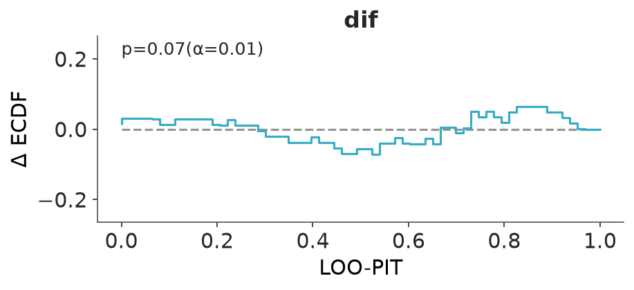
LOO-CV predictive checking for the continuous model indicates slight miscalibration with too many low PIT values (left tail of the predictive distribution is shorter than expected)
az.plot_loo_pit(idata_sqrt_c)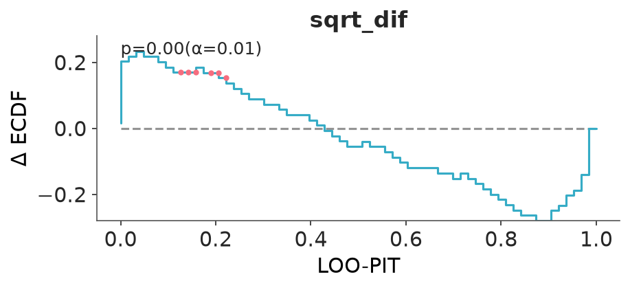
9 Bivariate Poisson and Poisson difference models
Bivariate Poisson model is commonly used for football scores Karlis and Ntzoufras (2003). If we care only about the score difference we can also use Poisson difference model Karlis and Ntzoufras (2003).
model_bipois = CmdStanModel(stan_file="worldcup_bivariate_poisson.stan")
print_stan(model_bipois)
functions {
real bivariate_poisson_log_lpmf_(int score1, int score2,
real log_lambda_1, real log_lambda_2, real log_lambda_3) {
// bivariate Poisson with lambda_3 presenting the correlation
// e.g. Karlis and Ntzoufras (2003). Analysis of sports data by using bivariate Poisson models
int m = min(score1, score2);
vector[m + 1] log_terms;
for (z in 0 : m) {
int r1 = score1 - z;
int r2 = score2 - z;
log_terms[z + 1] = r1 * log_lambda_1 - lgamma(r1 + 1)
+ r2 * log_lambda_2 - lgamma(r2 + 1)
+ z * log_lambda_3 - lgamma(z + 1);
}
return -exp(log_lambda_1) - exp(log_lambda_2) - exp(log_lambda_3) + log_sum_exp(log_terms);
}
real bivariate_poisson_log_lpmf(array[,] int score,
vector log_lambda_1, vector log_lambda_2, real log_lambda_3) {
// bivariate Poisson lpmf for array[2,N] scores
array[2] int score_dims = dims(score);
real total = 0;
for (i in 1:score_dims[2]) {
total += bivariate_poisson_log_lpmf_(score[1,i], score[2,i],
log_lambda_1[i], log_lambda_2[i], log_lambda_3);
}
return total;
}
real bivariate_poisson_log_lpmf(array[] int score,
real log_lambda_1, real log_lambda_2, real log_lambda_3) {
// bivariate Poisson lpmf for array[2] scores
return bivariate_poisson_log_lpmf_(score[1], score[2],
log_lambda_1, log_lambda_2, log_lambda_3);
}
}
data {
int N_teams;
int N_games;
vector[N_teams] prior_score;
array[N_games] int team_1;
array[N_games] int team_2;
array[N_games] int score_1;
array[N_games] int score_2;
}
parameters {
vector[N_teams] z_o;
vector[N_teams] z_d;
real a;
real b_o;
real b_d;
real c;
real<lower=0> sigma_o;
real<lower=0> sigma_d;
}
transformed parameters {
vector[N_teams] o = b_o * prior_score + sigma_o * z_o;
vector[N_teams] d = b_d * prior_score + sigma_d * z_d;
}
model {
z_o ~ normal(0, 1);
z_d ~ normal(0, 1);
b_o ~ normal(0, 1);
b_d ~ normal(0, 1);
a ~ normal(0, 1);
// prior centered on 1991–1992 Italian serie A data estimate as reported by
// Karlis and Ntzoufras (2003) and very wide prior around.
c ~ normal(-1.5, 20);
sigma_o ~ normal(0, 1);
sigma_d ~ normal(0, 1);
{score_1, score_2} ~ bivariate_poisson_log(a + o[team_1] + d[team_2],
a + o[team_2] + d[team_1],
c);
}
generated quantities {
array[N_games] int y_rep;
array[N_games] int score_1_rep;
array[N_games] int score_2_rep;
vector[N_games] log_lik;
vector[N_games] log_lik2;
for (n in 1:N_games) {
int score_c = poisson_log_rng(c);
score_1_rep[n] = poisson_log_rng(a + o[team_1[n]] + d[team_2[n]]) + score_c;
score_2_rep[n] = poisson_log_rng(a + o[team_2[n]] + d[team_1[n]]) + score_c;
y_rep[n] = score_1_rep[n] - score_2_rep[n];
// log probability using the bivariate Poisson lpmf
log_lik2[n] = bivariate_poisson_log_lpmf({score_1[n], score_2[n]} |
a + o[team_1[n]] + d[team_2[n]],
a + o[team_2[n]] + d[team_1[n]],
c);
// log probability using the Poisson difference lpmf
// note that lambda3 cancels out in the difference
int dif = score_1[n] - score_2[n];
real l1 = exp(o[team_1[n]] + d[team_2[n]]);
real l2 = exp(o[team_2[n]] + d[team_1[n]]);
log_lik[n] = -(l1 + l2) + (log(l1) - log(l2))*(dif/2.0) +
log(modified_bessel_first_kind(dif, 2.0*sqrt(l1*l2)));
}
}fit_bipois = model_bipois.sample(
data=stan_data, seed=SEED, show_progress=False, adapt_delta=0.95
)idata_bipois = az.from_cmdstanpy(
fit_bipois,
posterior_predictive="y_rep",
observed_data={"dif": dif},
log_likelihood={"dif": "log_lik"},
coords={"a_dim_0": teamnames},
)
idata_bipois.posterior_predictive.ds = idata_bipois.posterior_predictive.ds.rename({"y_rep": "dif", "y_rep_dim_0":"dif_dim_0"})
az.summary(idata_bipois, var_names=["a", "o", "d", "b_o", "b_d", "sigma_o", "sigma_d"])| mean | sd | eti90_lb | eti90_ub | ess_bulk | ess_tail | r_hat | mcse_mean | mcse_sd | |
|---|---|---|---|---|---|---|---|---|---|
| a | 0.08 | 0.23 | -0.41 | 0.33 | 345 | 443 | 1.01 | 0.014 | 0.015 |
| o[0] | 0.4 | 0.22 | 0.076 | 0.78 | 1378 | 1486 | 1.00 | 0.0061 | 0.0055 |
| o[1] | 0.32 | 0.23 | -0.065 | 0.69 | 1361 | 1419 | 1.00 | 0.0063 | 0.0054 |
| o[2] | 0.51 | 0.26 | 0.16 | 0.99 | 1047 | 1076 | 1.00 | 0.009 | 0.009 |
| o[3] | 0.31 | 0.23 | -0.063 | 0.7 | 1191 | 1261 | 1.00 | 0.0068 | 0.007 |
| ... | ... | ... | ... | ... | ... | ... | ... | ... | ... |
| d[31] | 0.45 | 0.263 | 0.047 | 0.9 | 3454 | 2674 | 1.00 | 0.0046 | 0.0038 |
| b_o | 0.51 | 0.23 | 0.18 | 0.94 | 612 | 767 | 1.00 | 0.0096 | 0.0084 |
| b_d | -0.438 | 0.191 | -0.76 | -0.13 | 2723 | 2478 | 1.00 | 0.0038 | 0.003 |
| sigma_o | 0.177 | 0.126 | 0.016 | 0.41 | 985 | 1582 | 1.00 | 0.0039 | 0.0036 |
| sigma_d | 0.28 | 0.16 | 0.036 | 0.57 | 327 | 825 | 1.01 | 0.0091 | 0.0074 |
69 rows × 9 columns
model_poisdif = CmdStanModel(stan_file="worldcup_poisson_difference.stan")
print_stan(model_poisdif)
data {
int N_teams;
int N_games;
vector[N_teams] prior_score;
array[N_games] int team_1;
array[N_games] int team_2;
vector[N_games] score_1;
vector[N_games] score_2;
}
transformed data {
vector[N_games] dif = score_1 - score_2;
}
parameters {
vector[N_teams] alpha;
real b;
real<lower=0> sigma_a;
}
transformed parameters {
vector[N_teams] a = b * prior_score + sigma_a * alpha;
}
model {
alpha ~ normal(0, 1);
b ~ normal(0, 1);
sigma_a ~ normal(0, 1);
for (n in 1:N_games) {
// log probability using the Poisson difference lpmf
// e.g. Karlis and Ntzoufras (2003). Analysis of sports data by using bivariate Poisson models
real l1 = exp(a[team_1[n]] - a[team_2[n]]);
real l2 = exp(a[team_2[n]] - a[team_1[n]]);
target += -(l1 + l2) + (log(l1) - log(l2))*(dif[n]/2.0) +
log(modified_bessel_first_kind(to_int(abs(dif[n])), 2.0*sqrt(l1*l2)));
}
}
generated quantities {
vector[N_games] y_rep;
vector[N_games] log_lik;
for (n in 1:N_games) {
int score_1_rep = poisson_log_rng(a[team_1[n]] - a[team_2[n]]);
int score_2_rep = poisson_log_rng(a[team_2[n]] - a[team_1[n]]);
y_rep[n] = score_1_rep - score_2_rep;
// log probability using the Poisson difference lpmf
// e.g. Karlis and Ntzoufras (2003). Analysis of sports data by using bivariate Poisson models
real l1 = exp(a[team_1[n]] - a[team_2[n]]);
real l2 = exp(a[team_2[n]] - a[team_1[n]]);
log_lik[n] = -(l1 + l2) + (log(l1) - log(l2))*(dif[n]/2.0) +
log(modified_bessel_first_kind(to_int(abs(dif[n])), 2.0*sqrt(l1*l2)));
}
}fit_poisdif = model_poisdif.sample(data=stan_data, seed=SEED,
inits=0.1, show_progress=False)idata_poisdif = az.from_cmdstanpy(
fit_poisdif,
posterior_predictive="y_rep",
observed_data={"dif": dif},
log_likelihood={"dif": "log_lik"},
coords={"a_dim_0": teamnames},
)
idata_poisdif.posterior_predictive.ds = idata_poisdif.posterior_predictive.ds.rename({"y_rep": "dif", "y_rep_dim_0":"dif_dim_0"})
az.summary(idata_poisdif, var_names=["a", "b", "sigma_a"])| mean | sd | eti90_lb | eti90_ub | ess_bulk | ess_tail | r_hat | mcse_mean | mcse_sd | |
|---|---|---|---|---|---|---|---|---|---|
| a[Bresil] | 0.227 | 0.206 | -0.13 | 0.54 | 4193 | 3264 | 1.00 | 0.0032 | 0.0023 |
| a[Argentine] | 0.396 | 0.182 | 0.099 | 0.7 | 6991 | 3351 | 1.00 | 0.0022 | 0.0016 |
| a[Allemagne] | 0.649 | 0.208 | 0.33 | 1 | 3254 | 2901 | 1.00 | 0.0036 | 0.0026 |
| a[Espagne] | 0.162 | 0.238 | -0.26 | 0.51 | 4387 | 2979 | 1.00 | 0.0036 | 0.0028 |
| a[Chili] | 0.314 | 0.21 | -0.045 | 0.66 | 6622 | 2967 | 1.00 | 0.0026 | 0.002 |
| a[France] | 0.417 | 0.203 | 0.1 | 0.77 | 5446 | 3324 | 1.00 | 0.0028 | 0.0021 |
| a[Colombie] | 0.414 | 0.198 | 0.12 | 0.75 | 4888 | 3263 | 1.00 | 0.0028 | 0.0022 |
| a[Uruguay] | 0.123 | 0.211 | -0.25 | 0.44 | 5781 | 3172 | 1.00 | 0.0028 | 0.0023 |
| a[Angleterre] | 0.081 | 0.228 | -0.32 | 0.42 | 5497 | 3339 | 1.00 | 0.0031 | 0.0026 |
| a[Belgique] | 0.205 | 0.189 | -0.098 | 0.52 | 8304 | 3348 | 1.00 | 0.0021 | 0.0017 |
| a[Pays-Bas] | 0.429 | 0.206 | 0.12 | 0.79 | 3171 | 2599 | 1.00 | 0.0036 | 0.0025 |
| a[Bosnie] | 0.079 | 0.207 | -0.28 | 0.41 | 7630 | 3162 | 1.00 | 0.0024 | 0.0019 |
| a[Equateur] | 0.063 | 0.21 | -0.29 | 0.41 | 6941 | 2941 | 1.00 | 0.0026 | 0.0022 |
| a[Portugal] | -0.013 | 0.213 | -0.37 | 0.32 | 6516 | 2746 | 1.00 | 0.0027 | 0.0022 |
| a[Coted'Ivoire] | -0.019 | 0.212 | -0.39 | 0.31 | 5429 | 2949 | 1.00 | 0.0029 | 0.0025 |
| a[Russie] | -0.058 | 0.211 | -0.42 | 0.27 | 6980 | 2680 | 1.00 | 0.0026 | 0.0021 |
| a[Italie] | -0.037 | 0.209 | -0.39 | 0.3 | 6578 | 2987 | 1.00 | 0.0026 | 0.0023 |
| a[Suisse] | -0.002 | 0.197 | -0.32 | 0.33 | 6950 | 3130 | 1.00 | 0.0024 | 0.0019 |
| a[Etats-Unis] | -0.018 | 0.197 | -0.33 | 0.32 | 7421 | 3511 | 1.00 | 0.0023 | 0.0019 |
| a[Mexique] | -0.009 | 0.197 | -0.33 | 0.32 | 5985 | 3177 | 1.00 | 0.0025 | 0.002 |
| a[Ghana] | -0.111 | 0.21 | -0.45 | 0.24 | 6919 | 3095 | 1.00 | 0.0026 | 0.0021 |
| a[Grece] | -0.176 | 0.202 | -0.51 | 0.15 | 8184 | 3500 | 1.00 | 0.0023 | 0.0018 |
| a[Croatie] | -0.175 | 0.213 | -0.52 | 0.18 | 7409 | 3393 | 1.00 | 0.0025 | 0.002 |
| a[Nigeria] | -0.167 | 0.204 | -0.49 | 0.18 | 6943 | 3237 | 1.00 | 0.0025 | 0.002 |
| a[Coree] | -0.301 | 0.214 | -0.66 | 0.033 | 7243 | 3393 | 1.00 | 0.0026 | 0.0022 |
| a[CostaRica] | -0.038 | 0.223 | -0.36 | 0.36 | 3740 | 3253 | 1.00 | 0.0036 | 0.0027 |
| a[Japon] | -0.351 | 0.217 | -0.72 | 0.0065 | 6422 | 3088 | 1.00 | 0.0027 | 0.0023 |
| a[Cameroun] | -0.552 | 0.239 | -0.98 | -0.19 | 3760 | 3063 | 1.00 | 0.0039 | 0.0029 |
| a[Iran] | -0.35 | 0.212 | -0.71 | 0.0051 | 8059 | 2915 | 1.00 | 0.0024 | 0.0019 |
| a[Honduras] | -0.504 | 0.226 | -0.89 | -0.15 | 5472 | 3169 | 1.00 | 0.0031 | 0.0023 |
| a[Algerie] | -0.229 | 0.232 | -0.57 | 0.18 | 4389 | 3279 | 1.00 | 0.0035 | 0.0027 |
| a[Australie] | -0.468 | 0.212 | -0.81 | -0.12 | 7467 | 3047 | 1.00 | 0.0025 | 0.0021 |
| b | 0.522 | 0.14 | 0.28 | 0.75 | 4742 | 3297 | 1.00 | 0.002 | 0.0015 |
| sigma_a | 0.235 | 0.091 | 0.082 | 0.39 | 1346 | 1390 | 1.00 | 0.0025 | 0.0019 |
The set in this case study is small, and we don’t see practical difference in the predictive performance.
az.compare({
    "Discrete": idata_discr,
    "Bivariate Poisson": idata_bipois,
    "Poisson difference": idata_poisdif,
})
/home/osvaldo/anaconda3/envs/bwb/lib/python3.14/site-packages/arviz_stats/loo/helper_loo.py:1146: UserWarning: Estimated shape parameter of Pareto distribution is greater than 0.70 for one or more samples. You should consider using a more robust model, this is because importance sampling is less likely to work well if the marginal posterior and LOO posterior are very different. This is more likely to happen with a non-robust model and highly influential observations.
warnings.warn(| rank | elpd_diff | dse | p_worse | diag_diff | diag_elpd | p | elpd | se | weight | |
|---|---|---|---|---|---|---|---|---|---|---|
| Poisson difference | 0 | 0.0 | 0.00 | NaN | 11.2 | -120.0 | 7.6 | 1.0 | ||
| Discrete | 1 | -1.0 | 1.60 | 0.81 | N < 100 | 11.7 | -120.0 | 8.2 | 0.0 | |
| Bivariate Poisson | 2 | -2.0 | 0.99 | 0.98 | N < 100 | 10 k̂ > 0.70 | 13.0 | -130.0 | 8.2 | 0.0 |
9.1 LOO-CV predictive checking
LOO-CV predictive checking with LOO-PIT for the binary Poisson model looks fine.
az.plot_loo_pit(idata_bipois)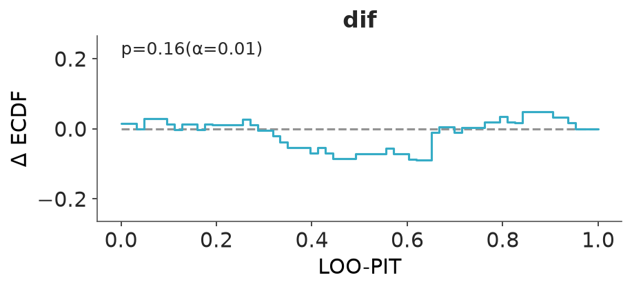
LOO-CV predictive checking with LOO-PIT for the Poisson difference model looks fine.
az.plot_loo_pit(idata_poisdif)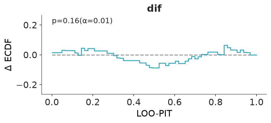
In this case study, we used many other models for illustration, but for real football score modeling, it is a good idea to start with the bivariate Poisson model. For real football analysis footBayes R package (Egidi, Macrì Demartino, and Palaskas 2025) has several different models including dynamic models allowing the latent performance to evolve in time.
References
Egidi, Leonardo, Roberto Macrì Demartino, and Vasilis Palaskas. 2025. footBayes: Fitting Bayesian and MLE Football Models. https://CRAN.R-project.org/package=footBayes.
Karlis, D., and I. Ntzoufras. 2003. “Analysis of Sports Data by Using Bivariate Poisson Models.” Journal of the Royal Statistical Society D 52: 381–93.
Silver, N. 2014. “It’s Brazil’s World Cup to Lose.” FiveThirtyEight.
Licenses
- Code © 2021–2025, Andrew Gelman, Aki Vehtari, licensed under BSD-3.
- Text © 2021–2025, Andrew Gelman, Aki Vehtari, licensed under CC-BY-NC 4.0.