---
title: "Declining exponentials"
image: ../social_cards/declining_exponentials.png
author: "Andrew Gelman"
date: 2022-08-15
date-modified: today
date-format: iso
format:
html:
number-sections: true
code-copy: true
code-download: true
code-tools: true
bibliography: ../casestudies.bib
---
This notebook includes the code for the Bayesian Workflow book
Section 12.4 *Using modeling ideas to address computing problems*.
## Introduction
- Declining exponential: A nonlinear model that comes up in many
science and engineering applications, also illustrating the use of
bounds in parameter estimation.
- Sum of declining exponentials: An important class of nonlinear
models that can be surprisingly difficult to estimate from data.
This example illustrates how inference/sampling can fail, and also the way in
which default prior information can add stability to an otherwise
intractable problem.
```{python}
#| label: setup
#| include: true
#| cache: false
import sys
import warnings

sys.path.insert(0, "..")

import numpy as np
import matplotlib.pyplot as plt
from cmdstanpy import CmdStanModel, disable_logging

import arviz as az

from utils import print_stan

warnings.filterwarnings("ignore")
disable_logging()

az.style.use("arviz-variat")
az.rcParams["stats.ci_prob"] = 0.95
plt.rcParams["figure.dpi"] = 100

SEED = 1123
rng = np.random.default_rng(SEED)
```
## Declining exponential
Let's fit the following simple model: $y = ae^{-bx} + \mathrm{error}$,
given data $(x,y)_i$:
$$
y_i = ae^{-bx_i} + \epsilon_i, \text{ for } i=1,\dots,N,
$$
We shall assume the errors are independent and normally
distributed: $\epsilon_i \sim \operatorname{normal}(0,\sigma)$.
Here is the model:
```{python}
#| output: asis
mod_1 = CmdStanModel(stan_file="exponential.stan")
print_stan(mod_1)
```
We have given the parameters $a$, and $b$, and $\sigma$ normal
prior distributions centered at 0 with standard deviation 10. In
addition, the parameter $\sigma$ is constrained to be positive.
The purpose of the prior distributions is to keep the computations
at a reasonable value. If we were working on a problem in which we
thought that $a$, $b$, or $\sigma$ could be much greater than 10,
we would want to use a weaker prior distribution.
### Simulated data
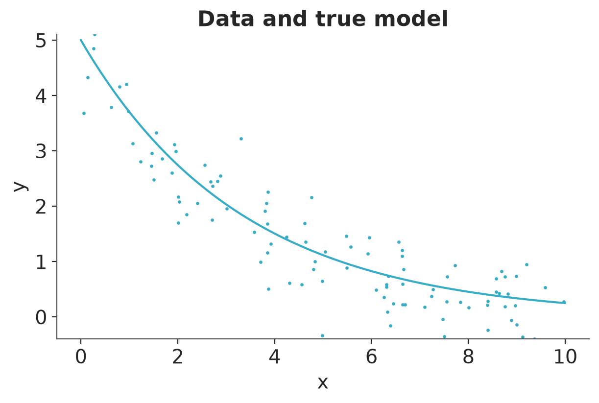
To demonstrate our exponential model, we fit it to fake data.
We'll simulate $N=100$ data points with predictors $x$ uniformly
distributed between 0 and 10, from the above model with $a=5$,
$b=0.3$, $\sigma=0.5$.
```{python}
a = 5
b = 0.3
sigma = 0.5
N = 100
x = rng.uniform(0, 10, N)
y = rng.normal(a * np.exp(-b * x), sigma)
```
Here is a graph of the true curve and the simulated data:
```{python}
#| label: fig-true-and-simulated
x_curve = np.linspace(0, 10, 200)
_, ax = plt.subplots(figsize=(6, 4))
ax.plot(x_curve, a * np.exp(-b * x_curve))
ax.scatter(x, y, s=2)
ax.set(
    xlabel="x",
    ylabel="y",
    ylim=(min(y.min(), 0), y.max()),
    title="Data and true model",
)
```
And then we fit the model:
```{python}
#| label: fit_1
#| results: hide
data_1 = {"N": N, "x": x, "y": y}
fit_1 = mod_1.sample(data=data_1, seed=SEED, show_progress=False)
```
Posterior summary:
```{python}
dt_1 = az.from_cmdstanpy(fit_1)
az.summary(dt_1)
```
Recall that the true parameter values were $a=5.0$, $b=0.3$,
$\sigma=0.5$. Here the model is simple enough and the data are
clean enough that we can estimate all three of these parameters
with reasonable precision from the data, as can be seen from the
95% intervals above.
Alternatively, we might want to say ahead of time that we are
fitting a declining exponential curve that starts positive and
descends to zero. We would thus want to constrain the parameters
$a$ and $b$ to be positive, which we can do in the parameters
block:
```
  real<lower=0> a;
  real<lower=0> b;
```
Otherwise we leave the model unchanged. In this case the results
turn out to be very similar:
```{python}
#| output: asis
mod_1b = CmdStanModel(stan_file="exponential_positive.stan")
print_stan(mod_1b)
```
```{python}
#| label: fit_1b
#| results: hide
fit_1b = mod_1b.sample(data=data_1, seed=SEED, show_progress=False)
```
Posterior summary:
```{python}
dt_1b = az.from_cmdstanpy(fit_1b)
az.summary(dt_1b)
```
### Small simulated data
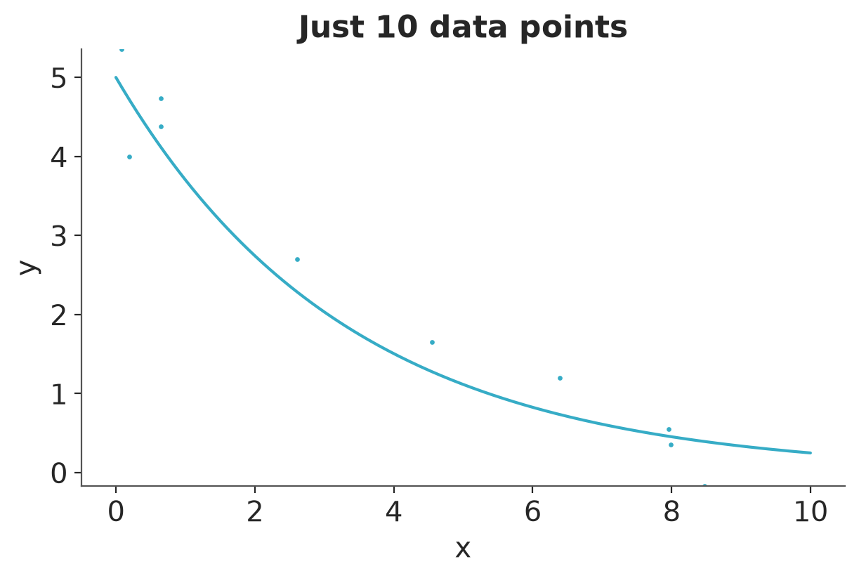
With weaker data, though, the constraints could make a difference.
We could experiment on this by doing the same simulation but with
just $N=10$ data points:
```{python}
a = 5
b = 0.3
sigma = 0.5
N = 10
x = rng.uniform(0, 10, N)
y = rng.normal(a * np.exp(-b * x), sigma)
```
```{python}
#| label: fig-10-data-points
x_curve = np.linspace(0, 10, 200)
_, ax = plt.subplots(figsize=(6, 4))
ax.plot(x_curve, a * np.exp(-b * x_curve))
ax.scatter(x, y, s=2)
ax.set(
    xlabel="x",
    ylabel="y",
    ylim=(min(y.min(), 0), y.max()),
    title="Just 10 data points",
)
```
First we fit the unconstrained model:
```{python}
#| label: fit_2
#| results: hide
data_2 = {"N": N, "x": x, "y": y}
fit_2 = mod_1.sample(data=data_2, seed=SEED, show_progress=False)
```
Posterior summary:
```{python}
dt_2 = az.from_cmdstanpy(fit_2)
az.summary(dt_2)
```
Then we fit the constrained model:
```{python}
#| label: fit_2b
#| results: hide
fit_2b = mod_1b.sample(data=data_2, seed=SEED, show_progress=False)
```
Posterior summary:
```{python}
dt_2b = az.from_cmdstanpy(fit_2b)
az.summary(dt_2b)
```
Different things can happen with different sets of simulated data,
but the inference with the positivity constraints will typically be
much more stable. Of course, we would only want to constrain the
model in this way if we knew that the positivity restriction is
appropriate.
### Positive simulated data
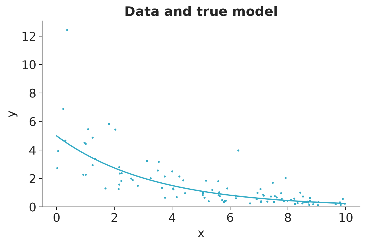
Now suppose that the data are also restricted to be positive. Then
we need a different error distribution, as the above model with
additive normal errors can yield negative data.
Let's try a multiplicative error, with a lognormal distribution:
$$
y_i = ae^{-bx_i} \cdot \epsilon_i, \text{ for } i=1,\dots,N\\
\log\epsilon_i \sim \operatorname{normal}(0,\log\sigma), \text{ for } i=1,\dots,N
$$
Here is the model:
```{python}
#| output: asis
mod_3 = CmdStanModel(stan_file="exponential_positive_lognormal.stan")
print_stan(mod_3)
```
As before, we can simulate fake data from this model:
```{python}
a = 5
b = 0.3
sigma = 0.5
N = 100
x = rng.uniform(0, 10, N)
epsilon = np.exp(rng.normal(0, sigma, N))
y = a * np.exp(-b * x) * epsilon
```
```{python}
#| label: fig-positive-true-and-simulated
x_curve = np.linspace(0, 10, 200)
_, ax = plt.subplots(figsize=(6, 4))
ax.plot(x_curve, a * np.exp(-b * x_curve))
ax.scatter(x, y, s=2)
ax.set(
    xlabel="x",
    ylabel="y",
    ylim=(0, y.max() * 1.05),
    title="Data and true model",
)
```
We can then fit the model to the simulated data and check that the
parameters are approximately recovered:
```{python}
#| label: fit_3
#| results: hide
data_3 = {"N": N, "x": x, "y": y}
fit_3 = mod_3.sample(data=data_3, seed=SEED, show_progress=False)
```
Posterior summary:
```{python}
dt_3 = az.from_cmdstanpy(fit_3)
az.summary(dt_3)
```
## Sum of declining exponentials
From the numerical analysis literature, here is an example of an
inference problem that appears simple but can be surprisingly
difficult. The challenge is to estimate the parameters of a sum of
declining exponentials: $y = a_1e^{-b_1x} + a_2e^{-b_2x}$. This is
also called an inverse problem, and it can be challenging to
decompose these two declining functions.
This expression, and others like it, arise in many examples,
including in pharmacology, where $x$ represents time and $y$ could
be the concentration of a drug in the blood of someone who was
given a specified dose at time 0. In a simple _two-compartment
model_, the total concentration will look like a sum of declining
exponentials.
To set this up as a statistics problem, we add some noise to the
system. We want the data to always be positive so our noise will be
multiplicative:
$$
y_i = (a_1e^{-b_1x_i} + a_2e^{-b_2x_i}) \cdot \epsilon_i, \text{ for } i=1,\dots,N,
$$
with lognormally-distributed errors $\epsilon$.
Here is the model:
```{python}
#| output: asis
mod_4 = CmdStanModel(stan_file="sum_of_exponentials.stan")
print_stan(mod_4)
```
The coefficients $a$ and the residual standard deviation $\sigma$
are constrained to be positive. The parameters $b$ are also
positive---these are supposed to be declining, not increasing,
exponentials---and are also constrained to be ordered, so that
$b_1<b_2$. We need this to keep the model _identified_: Without
some sort of restriction, there would be no way from the data to
tell which component is labeled 1 and which is 2. So we
arbitrarily label the component with lower value of $b$---that is,
the one that declines more slowly---as the first one, and the
component with higher value of $b$ to be the second. We added the
`positive_ordered` type to Stan because this sort of identification
problem comes up fairly often in applications.
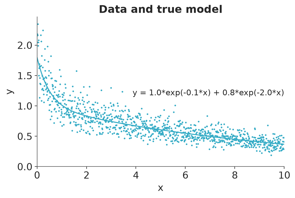
We'll try out our model by simulating fake data from a model
where the two curves should be cleanly distinguished, setting
$b_1=0.1$ and $b_2=2.0$, a factor of 20 apart in scale. We'll
simulate 1000 data points where the predictors $x$ are uniformly
spaced from 0 to 10, and, somewhat arbitrarily, set $a_1=1.0$,
$a_2=0.8$, and $\sigma=0.2$. We can then simulate from the
lognormal distribution to generate the data $y$.
```{python}
a = np.array([1.0, 0.8])
b = np.array([0.1, 2.0])
N = 1000
x = np.linspace(0, 10, N)
sigma = 0.2
epsilon = np.exp(rng.normal(0, sigma, N))
y = (a[0] * np.exp(-b[0] * x) + a[1] * np.exp(-b[1] * x)) * epsilon
```
Here is a graph of the true curve and the simulated data:
```{python}
#| label: fig-sumexp-true-and-simulated
x_curve = np.linspace(0, 10, 200)
y_true = a[0] * np.exp(-b[0] * x_curve) + a[1] * np.exp(-b[1] * x_curve)
_, ax = plt.subplots(figsize=(6, 4))
ax.plot(x_curve, y_true)
ax.scatter(x, y, s=2)
ax.set(
    xlabel="x",
    ylabel="y",
    xlim=(0, 10),
    ylim=(0, y.max() * 1.05),
    title="Data and true model",
)
label = f"y = {a[0]:.1f}*exp({-b[0]:.1f}*x) + {a[1]:.1f}*exp({-b[1]:.1f}*x)"
ax.text(x_curve[-1], 0.5 * y.max(), label, ha="right")
```
And then we fit the model:
```{python}
#| label: fit_4
#| results: hide
data_4 = {"N": N, "x": x, "y": y}
fit_4 = mod_4.sample(data=data_4, seed=SEED, show_progress=False)
```
Posterior summary:
```{python}
dt_4 = az.from_cmdstanpy(fit_4)
az.summary(dt_4)
```
The parameters are recovered well, with the only difficulty being
$b_2$, where the estimate is 1.89 but the true value is 2.0---but
that is well within the posterior uncertainty. Inference worked just
fine on this nonlinear model.
But now let's make the problem just slightly more difficult.
Instead of setting the two parameters $b$ to 0.1 and 2.0, we'll
make them 0.1 and 0.2, so now only a factor of 2 separates the
scales of the two declining exponentials.
```{python}
b = np.array([0.1, 0.2])
y_2 = (a[0] * np.exp(-b[0] * x) + a[1] * np.exp(-b[1] * x)) * epsilon
data_5 = {"N": N, "x": x, "y": y_2}
```
This should still be easy to fit, right? Wrong:
```{python}
#| label: fit_5
#| results: hide
fit_5 = mod_4.sample(data=data_5, seed=SEED, show_progress=False)
```
Posterior summary:
```{python}
dt_5 = az.from_cmdstanpy(fit_5)
az.summary(dt_5, round_to="None")
```
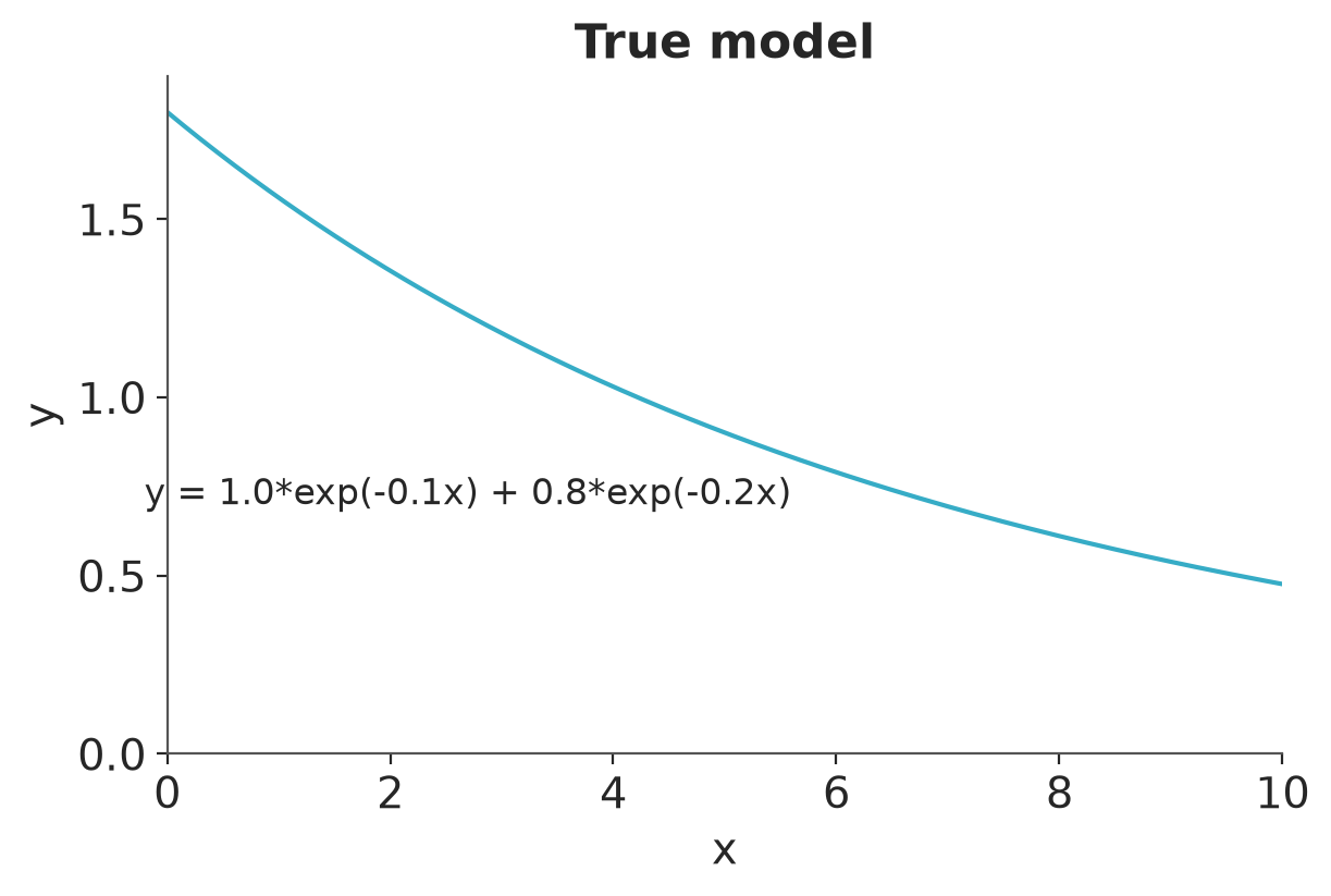
What happened?? It turns out that these two declining exponentials
are _very_ hard to detect. Look: here's a graph of the
two-component model for the expected data,
$y=1.0e^{-0.1x}+0.8e^{-0.2x}$:
```{python}
#| label: fig-sumexp-true-model
a_true = np.array([1.0, 0.8])
b_true = np.array([0.1, 0.2])
x_curve = np.linspace(0, 10, 200)
_, ax = plt.subplots(figsize=(6, 4))
y_true = a_true[0] * np.exp(-b_true[0] * x_curve) + a_true[1] * np.exp(-b_true[1] * x_curve)
ax.plot(x_curve, y_true)
ax.set(
    xlabel="x",
    ylabel="y",
    xlim=(0, 10),
    ylim=(0, 1.9),
    title="True model",
)
ax.text(5.6, 0.7, "y = 1.0*exp(-0.1x) + 0.8*exp(-0.2x)", ha="right")
```
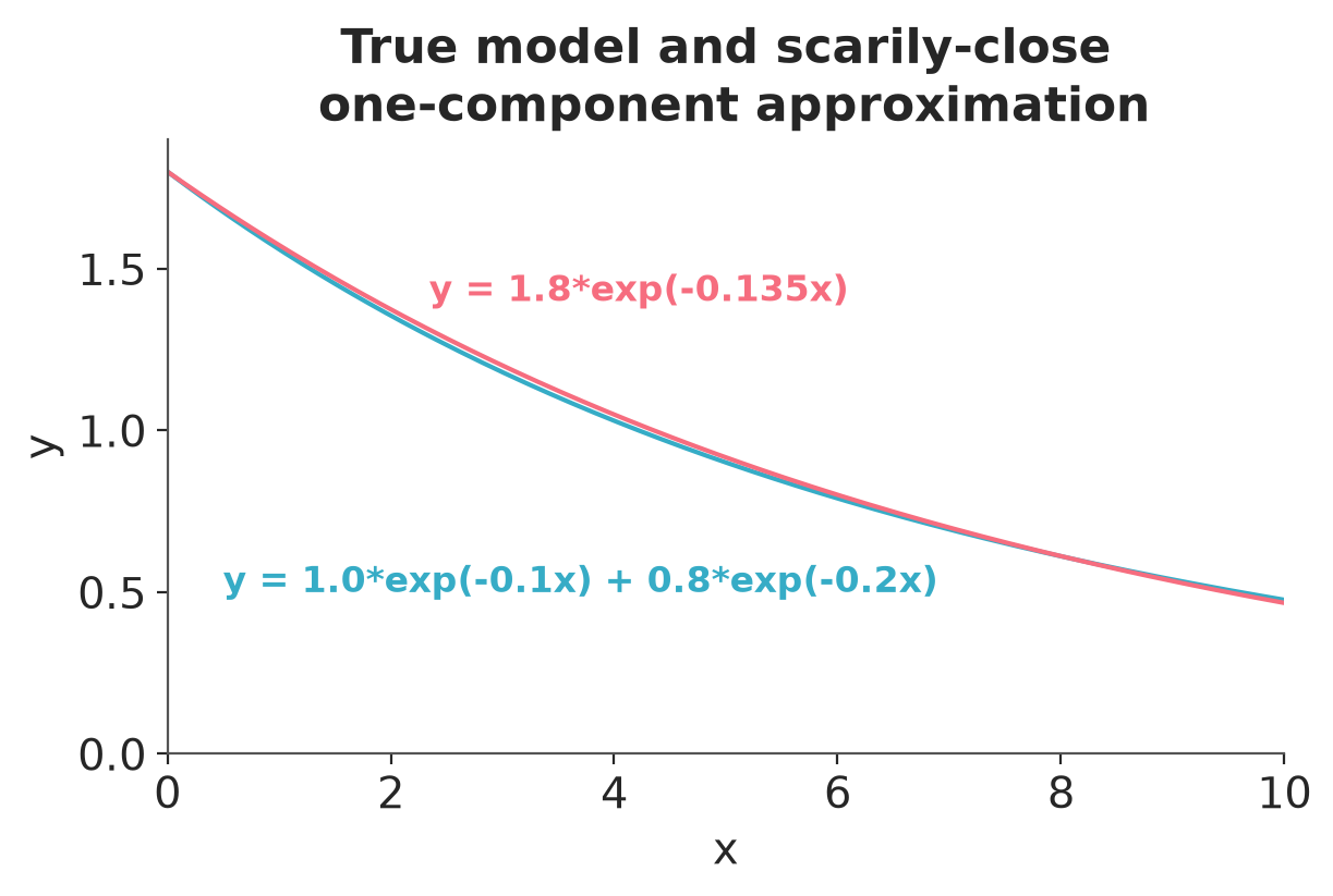
And now we'll overlay a graph of a particular _one-component_ model,
$y=1.8e^{-0.135x}$:
```{python}
#| label: fig-sumexp-true-and-one-component
_, ax = plt.subplots(figsize=(6, 4))
y_true = a_true[0] * np.exp(-b_true[0] * x_curve) + a_true[1] * np.exp(-b_true[1] * x_curve)
ax.plot(x_curve, y_true)
ax.plot(x_curve, 1.8 * np.exp(-0.135 * x_curve))
ax.set(
    xlabel="x",
    ylabel="y",
    xlim=(0, 10),
    ylim=(0, 1.9),
)
ax.set_title("True model and scarily-close\n one-component approximation",
)
ax.text(6.9, 0.5, "y = 1.0*exp(-0.1x) + 0.8*exp(-0.2x)", ha="right", color="C0", fontdict={"weight": "bold"});
ax.text(6.1, 1.4, "y = 1.8*exp(-0.135x)", ha="right", color="C1", fontdict={"weight": "bold"});
```
The two lines are strikingly close, and it would be essentially
impossible to tell them apart based on noisy data, even 1000
measurements. So we had trouble recovering the true parameters
from the data.
Still, if the parameters are difficult to fit, this should just
result in a high posterior uncertainty. Why did the fit
explode? The problem in this case is that, since only one term in
the model was required to fit these data, the second term was
completely free---and the parameter $\beta_2$ was unbounded: there
was nothing stopping it from being estimated as arbitrarily large.
This sort of unbounded posterior distribution is called _improper_
(see Bayesian Data Analysis for a more formal definition), and
there is no way of drawing simulations from such a distribution,
hence sampling does not converge. The simulations drift off to
infinity, as there is nothing in the prior or likelihood that is
keeping them from doing so.
To fix the problem, we can add some prior information. Here we
shall use our default, which is independent $\operatorname{normal}(0,1)$
prior densities on all the parameters; thus, we add these lines to
the model:
```
  a ~ normal(0, 1);
  b ~ normal(0, 1);
  sigma ~ normal(0, 1);
```
For this particular example, all we really need is a prior on $b$
(really, just $b_2$ because of the ordering), but to demonstrate
the point we shall assign default priors to everything. The priors
are in addition to the rest of the model; that is, they go on top
of the positivity and ordering constraints. So, for example, the
prior for $\sigma$ is the positive half of a normal, which is
sometimes written as $\operatorname{normal}^+(0,1)$.
We now can fit this new model to our data, and the results are much
more stable:
```{python}
#| output: asis
mod_5_with_priors = CmdStanModel(stan_file="sum_of_exponentials_with_priors.stan")
print_stan(mod_5_with_priors)
```
```{python}
#| label: fit_5_with_priors
#| results: hide
fit_5_with_priors = mod_5_with_priors.sample(data=data_5, seed=SEED, show_progress=False)
```
Posterior summary:
```{python}
dt_5_with_priors = az.from_cmdstanpy(fit_5_with_priors)
az.summary(dt_5_with_priors)
```
The fit is far from perfect---compare to the true parameter values,
$a_1=1.0$, $a_2=0.8$, $b_1=0.1$, $b_2=0.2$---but we have to expect
that. As explained above, the data at hand do not identify the
parameters, so all we can hope for in a posterior distribution is
some summary of uncertainty.
The question then arises, what about those prior distributions? We
can think about them in a couple different ways.
From one direction, we can think of scaling. We are using priors
centered at 0 with a scale of 1; this can be reasonable if the
parameters are on "unit scale," meaning that we expect them to be
of order of magnitude around 1. Not all statistical models are on
unit scale. For example, in the above model, if the data $y_i$ are
on unit scale, but the data values $x_i$ take on values in the
millions, then we'd probably expect the parameters $b_1$ and $b_2$
to be roughly on the scale of $10^{-6}$. In such a case, we'd want
to rescale $x$ so that the coefficients $b$ are more interpretable.
Similarly, if the values of $y$ ranged in the millions, then the
coefficients $a$ would have to be of order $10^6$, and, again, we
would want to rescale the data or the model so that $a$ would be on
unit scale. By using unit scale priors, we are implicitly assuming
the model has been scaled.
From the other direction, instead of adapting the model to the
prior distribution, we could adapt the prior to the model. That
would imply an understanding of a reasonable range of values for
the parameters, based on the context of the problem. In any
particular example this could be done by simulating parameter
vectors from the prior distribution and graphing the corresponding
curves of expected data, and seeing if these could plausibly cover
the possible cases that might arise in the particular problem being
studied.
No matter how it's done, inference has to come from somewhere, and
if the data are weak, you need to put in prior information if your
goal is to make some statement about possible parameter values, and
from there to make probabilistic predictions and decisions.
<br />
## Licenses {.unnumbered}
* Code © 2022--2025, Andrew Gelman, licensed under BSD-3.
* Text © 2022--2025, Andrew Gelman, licensed under CC-BY-NC 4.0.