---
title: "Simulated data of movie ratings"
image: ../social_cards/movies.png
author: "Andrew Gelman and Aki Vehtari"
date: 2022-08-15
date-modified: today
date-format: iso
format:
html:
number-sections: true
code-copy: true
code-download: true
code-tools: true
bibliography: ../casestudies.bib
---
This notebook includes the code for the Bayesian Workflow book
Chapter 16 *Coding a series of models: Simulated data of movie
ratings*.
## Introduction
Consider the following scenario. You are considering which of two
movies to go see. Both have average online ratings of 4 out of 5
stars, but one is based on 2 ratings and the other is based on 100.
Which movie should you choose?
**Load packages**
```{python}
#| label: setup
#| include: true
#| cache: false
import sys
import warnings
sys.path.insert(0, '..')

import arviz as az
import matplotlib.pyplot as plt
import numpy as np
import pandas as pd
import xarray as xr
from cmdstanpy import CmdStanModel, disable_logging

from utils import print_stan

warnings.filterwarnings("ignore")
disable_logging()

az.style.use("arviz-variat")
az.rcParams["stats.ci_prob"] = 0.95
plt.rcParams["figure.dpi"] = 100
SEED = 1234
rng = np.random.default_rng(SEED)
```
## Model for two movies
```{python}
y_1 = np.array([3, 5])
y_2 = np.repeat([2, 3, 4, 5], [10, 20, 30, 40])
y = np.concatenate([y_1, y_2])
N = len(y)
movie = np.repeat([1, 2], [len(y_1), len(y_2)])
movie_data = {"y": y, "N": N, "movie": movie}
```
```{python}
mod_1 = CmdStanModel(stan_file="ratings_1.stan")
print_stan(mod_1)
```
Sample
```{python}
#| label: fit_1
#| results: hide
fit_1 = mod_1.sample(data=movie_data, seed=SEED, show_progress=False)
```
```{python}
idata_1 = az.from_cmdstanpy(fit_1)
```
Posterior summary
```{python}
az.summary(idata_1, var_names=["theta", "sigma_y"])
```
## Extending the model to J movies
```{python}
J = 40
N_ratings = rng.integers(0, 101, size=J)
N = N_ratings.sum()
movie = np.repeat(np.arange(1, J + 1), N_ratings)
theta_true = rng.normal(3.0, 0.5, size=J)
y = rng.normal(np.repeat(theta_true, N_ratings), 2.0)
movie_data = {"y": y, "N": N, "J": J, "movie": movie}
```
```{python}
mod_2 = CmdStanModel(stan_file="ratings_2.stan")
print_stan(mod_2)
```
Sample
```{python}
#| label: fit_2
#| results: hide
fit_2 = mod_2.sample(data=movie_data, seed=SEED, show_progress=False)
```
```{python}
idata_2 = az.from_cmdstanpy(fit_2)
```
Posterior summary
```{python}
az.summary(idata_2, var_names=["theta", "sigma_y"]).head()
```
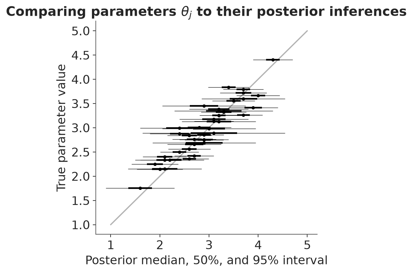
Comparing parameters $\theta_j$ to their posterior inferences
```{python}
#| label: fig-movies_1
median =az.median(idata_2.posterior["theta"])
q_50 =az.iqr(idata_2.posterior["theta"])
q_95 =az.iqr(idata_2.posterior["theta"], quantiles=[0.025, 0.975])

_, ax = plt.subplots(figsize=(4.5, 4.5))
ax.errorbar(median, theta_true, xerr=q_50/2, color="k", lw=2, fmt=".")
ax.errorbar(median, theta_true, xerr=q_95/2, color="k", lw=0.5, fmt="none")
ax.plot([1, 5], [1, 5], color="0.7", zorder=-1)
ax.set(xlabel="Posterior median, 50%, and 95% interval",
       ylabel="True parameter value",
       title="Comparing parameters $\\theta_j$ to their posterior inferences");
```
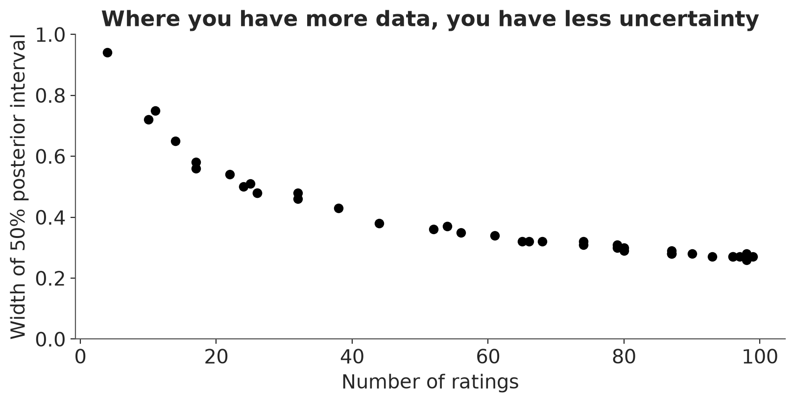
Where you have more data, you have less uncertainty
```{python}
#| label: fig-movies_2
#| fig-height: 4
#| fig-width: 6
_, ax = plt.subplots(figsize=(8, 4))
ax.plot(N_ratings, q_50, "ko")
ax.set(ylim=(0, 1),
       xlabel="Number of ratings",
       ylabel="Width of 50% posterior interval",
       title="Where you have more data, you have less uncertainty");
```
## Item-response model with parameters for raters and for movies
### Balanced data
```{python}
J = 40
K = 100
N = J * K
movie = np.repeat(np.arange(1, J + 1), K)
rater = np.tile(np.arange(1, K + 1), J)
mu = 3
sigma_a = 0.5
sigma_b = 0.5
sigma_y = 2
alpha_true = rng.normal(0, 1, size=J)
beta_true = rng.normal(0, 1, size=K)
y = rng.normal(mu + sigma_a * alpha_true[movie - 1] - sigma_b * beta_true[rater - 1], sigma_y)
data_3 = {"N": N, "J": J, "K": K, "movie": movie, "rater": rater, "y": y}
```
```{python}
mod_3 = CmdStanModel(stan_file="ratings_3.stan")
print_stan(mod_3)
```
Sample
```{python}
#| label: fit_3
#| results: hide
fit_3 = mod_3.sample(data=data_3, seed=SEED, show_progress=False)
```
```{python}
idata_3 = az.from_cmdstanpy(fit_3)
```
Posterior summary
```{python}
az.summary(idata_3, var_names=["mu", "sigma_a", "sigma_b", "sigma_y"])
```
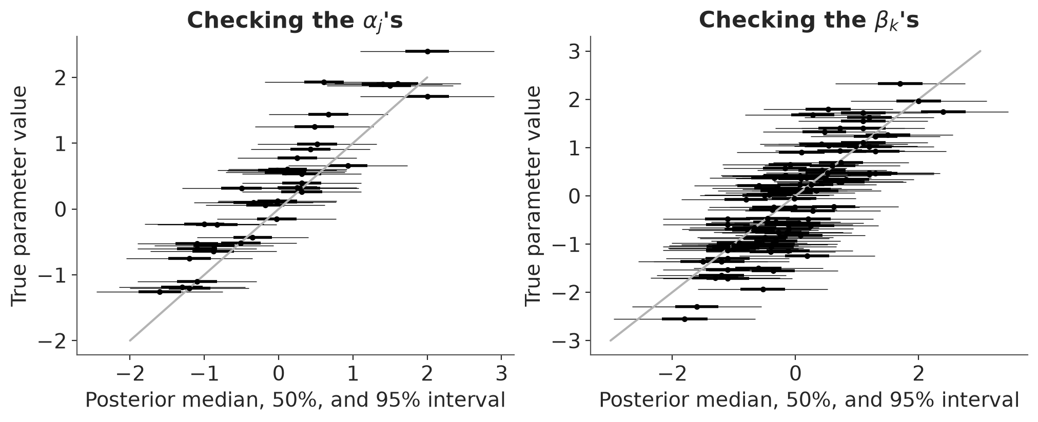
Checking the $\alpha_j$'s and $\beta_k$'s
```{python}
#| label: fig-movies_3
alpha_median = az.median(idata_3.posterior["alpha"])
alpha_q50 = az.iqr(idata_3.posterior["alpha"])
alpha_q90 = az.iqr(idata_3.posterior["alpha"], quantiles=[0.025, 0.975])
beta_median = az.median(idata_3.posterior["beta"])
beta_q50 = az.iqr(idata_3.posterior["beta"])
beta_q90 = az.iqr(idata_3.posterior["beta"], quantiles=[0.025, 0.975])

_, axes = plt.subplots(1, 2, figsize=(10, 4))

axes[0].errorbar(alpha_median, alpha_true, xerr=alpha_q50/2, color="k", lw=2, fmt=".")
axes[0].errorbar(alpha_median, alpha_true, xerr=alpha_q90/2, color="k", lw=0.5, fmt="none")
axes[0].plot([-2, 2], [-2, 2], color="0.7")
axes[0].set(xlabel="Posterior median, 50%, and 95% interval",
            ylabel="True parameter value",
            title="Checking the $\\alpha_j$'s")


axes[1].errorbar(beta_median, beta_true, xerr=beta_q50/2, color="k", lw=2, fmt=".")
axes[1].errorbar(beta_median, beta_true, xerr=beta_q90/2, color="k", lw=0.5, fmt="none")
axes[1].plot([-3, 3], [-3, 3], color="0.7")
axes[1].set(xlabel="Posterior median, 50%, and 95% interval",
            ylabel="True parameter value",
            title="Checking the $\\beta_k$'s");
```
### Unbalanced data
```{python}
genre = np.array(["romantic"] * (J // 2) + ["crime"] * (J - J // 2))
prob_of_rated = np.where(beta_true[rater - 1] > 0,
                         np.where(genre[movie - 1] == "romantic", 0.2, 0.7),
                         np.where(genre[movie - 1] == "romantic", 0.7, 0.2))
rated = rng.random(N) < prob_of_rated
data_3a = {"N": rated.sum(), "J": J, "K": K,
           "movie": movie[rated], "rater": rater[rated],
           "y": y[rated]}
```
Sample
```{python}
#| label: fit_3a
#| results: hide
fit_3a = mod_3.sample(data=data_3a, seed=SEED, show_progress=False)
```
```{python}
idata_3a = az.from_cmdstanpy(fit_3a)
```
Posterior summary
```{python}
az.summary(idata_3a, var_names=["mu", "sigma_a", "sigma_b", "sigma_y"])
```
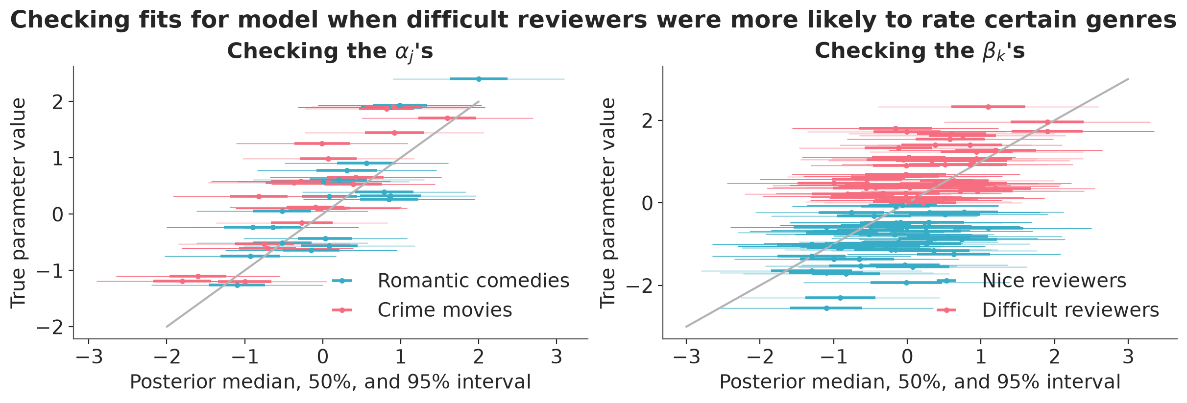
Checking fits for model when difficult reviewers were more likely to rate certain genres
```{python}
#| label: fig-movies_4
#| fig-height: 4
#| fig-width: 8
alpha_median = az.median(idata_3a.posterior["alpha"])
alpha_q50 = az.iqr(idata_3a.posterior["alpha"])
alpha_q95 = az.iqr(idata_3a.posterior["alpha"], quantiles=[0.025, 0.975])
beta_median = az.median(idata_3a.posterior["beta"])
beta_q50 = az.iqr(idata_3a.posterior["beta"])
beta_q95 = az.iqr(idata_3a.posterior["beta"], quantiles=[0.025, 0.975])

fig, axes = plt.subplots(1, 2, figsize=(12, 4))


romantic_mask = genre == "romantic"
crime_mask = genre == "crime"

axes[0].errorbar(alpha_median[romantic_mask], alpha_true[romantic_mask], xerr=alpha_q50[romantic_mask]/2, color="C0", lw=2, fmt=".", label="Romantic comedies")
axes[0].errorbar(alpha_median[crime_mask], alpha_true[crime_mask], xerr=alpha_q50[crime_mask]/2, color="C1", lw=2, fmt=".", label="Crime movies")

axes[0].errorbar(alpha_median[romantic_mask], alpha_true[romantic_mask], xerr=alpha_q95[romantic_mask]/2, color="C0", lw=0.5, fmt="none")
axes[0].errorbar(alpha_median[crime_mask], alpha_true[crime_mask], xerr=alpha_q95[crime_mask]/2, color="C1", lw=0.5, fmt="none")

axes[0].set(xlabel="Posterior median, 50%, and 95% interval",
            ylabel="True parameter value",
            title="Checking the $\\alpha_j$'s")
axes[0].plot([-2, 2], [-2, 2], color="0.7")
axes[0].legend(loc="lower right", frameon=False)

nice_mask = beta_true < 0
difficult_mask = beta_true > 0

axes[1].errorbar(beta_median[nice_mask], beta_true[nice_mask], xerr=beta_q50[nice_mask]/2, color="C0", lw=2, fmt=".", label="Nice reviewers")
axes[1].errorbar(beta_median[difficult_mask], beta_true[difficult_mask], xerr=beta_q50[difficult_mask]/2, color="C1", lw=2, fmt=".", label="Difficult reviewers")

axes[1].errorbar(beta_median[nice_mask], beta_true[nice_mask], xerr=beta_q95[nice_mask]/2, color="C0", lw=0.5, fmt="none")
axes[1].errorbar(beta_median[difficult_mask], beta_true[difficult_mask], xerr=beta_q95[difficult_mask]/2, color="C1", lw=0.5, fmt="none")

axes[1].set(xlabel="Posterior median, 50%, and 95% interval",
            ylabel="True parameter value",
            title="Checking the $\\beta_k$'s")
axes[1].plot([-3, 3], [-3, 3], color="0.7")
axes[1].legend(loc="lower right", frameon=False)

fig.suptitle("Checking fits for model when difficult reviewers were more likely to rate certain genres");
```
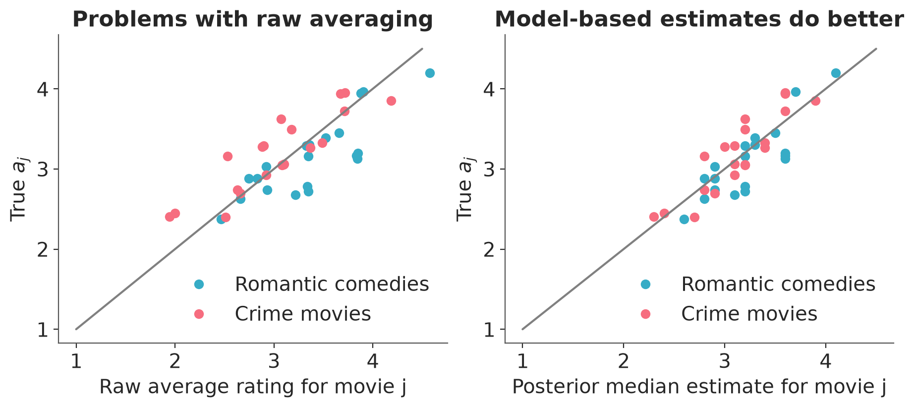
## Comparison to naive data averaging
```{python}
ybar = np.array([y[(movie == j) & rated].mean() for j in range(1, J + 1)])
a_true = mu + sigma_a * alpha_true
a_post_median = az.median(idata_3a)["a"]
```
```{python}
#| label: fig-movies_5
_, axes = plt.subplots(1, 2, figsize=(9, 4))

axes[0].plot(ybar[romantic_mask], a_true[romantic_mask],
                "C0o", label="Romantic comedies")
axes[0].plot(ybar[crime_mask], a_true[crime_mask],
                "C1o", label="Crime movies")
axes[0].set(xlabel="Raw average rating for movie j",
            ylabel="True $a_j$",
            title="Problems with raw averaging")
axes[0].plot([1, 4.5], [1, 4.5], color="gray")

axes[0].legend(loc="lower right", frameon=False)

axes[1].plot(a_post_median[romantic_mask], a_true[romantic_mask],
                "C0o", label="Romantic comedies")
axes[1].plot(a_post_median[crime_mask], a_true[crime_mask],
                "C1o", label="Crime movies")
axes[1].set(xlabel="Posterior median estimate for movie j",
            ylabel="True $a_j$",
            title="Model-based estimates do better")
axes[1].plot([1, 4.5], [1, 4.5], color="gray")

axes[1].legend(loc="lower right", frameon=False);
```
<br />
## References {.unnumbered}
<div id="refs"></div>
## Licenses {.unnumbered}
* Code © 2022--2025, Andrew Gelman, licensed under BSD-3.
* Text © 2022--2025, Andrew Gelman, licensed under CC-BY-NC 4.0.