Posterior predictive checking: Stochastic learning in dogs

This notebook includes the Bambi code for the Bayesian Workflow book Chapter 21 Posterior predictive checking: Stochastic learning in dogs.

1 Introduction

This notebook is a remake of Andrew Gelman’s analysis of stochastic learning in dogs data by Bush and Mosteller (1955). Andrew wrote his models in Stan language, and here we use Bambi and add some further diagnostics.

import sys
import warnings

sys.path.insert(0, "..")

import numpy as np
import pandas as pd
import matplotlib.pyplot as plt
from matplotlib.colors import ListedColormap
from scipy.special import expit, logit

import bambi as bmb
import arviz as az

warnings.filterwarnings("ignore")

az.style.use("arviz-variat")
az.rcParams["stats.ci_prob"] = 0.95
plt.rcParams["figure.dpi"] = 100

SEED = 123
rng = np.random.default_rng(SEED)

shock_cmap = ListedColormap(["#fac364", "#7c2695"])

2 Data

Data comes originally from a book by Bush and Mosteller (1955). The data come from 30 dogs in a stochastic learning experiment. Each dog was put in a cage where it would be shocked if it did not jump out in time, a few seconds after a light goes on (we do not advocate giving shocks to dogs). After 25 tries, all of the dogs learned to jump and avoid the shock. Bush and Mosteller then posited a two-parameter model which allowed different amounts of learning from shocks and avoidances:

\[ \Pr(\mathrm{shock}) = a^\mathrm{(\# \ of \ previous \ shocks)}\, b^\mathrm{(\# \ of \ previous \ avoidances)} \]

Under this model, the probability of being shocked starts at 1, which is appropriate, as there is no reason the dogs should know at the start that the light would precede a shock, and indeed any dogs that jumped before the first trial were excluded from the experiment. From then on, as long as the parameters \(a\) and \(b\) are between 0 and 1, the probability of shock gradually declines over time.

dogs_raw = pd.read_csv("data/dogs.dat", skiprows=2, sep=r"\s+", header=None)
shock_matrix = (dogs_raw.iloc[:, 2:26].values == "S").astype(int)

n_dogs, n_trials = shock_matrix.shape

dogs_df = pd.DataFrame({
    "shock": shock_matrix.ravel(),
    "dog": np.repeat(np.arange(1., n_dogs + 1), n_trials),
    "time": np.tile(np.arange(1, n_trials + 1), n_dogs),
})

dogs_df = dogs_df[dogs_df["time"] > 1].reset_index(drop=True)

prev_shock_cumsum = np.cumsum(shock_matrix, axis=1)[:, :-1]
prev_avoid_cumsum = np.cumsum(1 - shock_matrix, axis=1)[:, :-1]
dogs_df["prev_shock"] = prev_shock_cumsum.ravel().astype(float)
dogs_df["prev_avoid"] = prev_avoid_cumsum.ravel().astype(float)

3 Model 0: Logistic regression

We start with a simple logistic regression model

\[ \Pr(\mathrm{shock}) = \mathrm{logit}^{-1}(\alpha + \beta t) \]

where \(t\) denotes time. We assign priors:

\[ \begin{aligned} \alpha &\sim \mathrm{Student}_3(0, 2.5)\\ \beta &\sim \mathrm{normal}(0, 1). \end{aligned} \]

model_0 = bmb.Model(
    "shock ~ time",
    data=dogs_df,
    family="bernoulli",
    priors={"Intercept": bmb.Prior("StudentT", nu=3, mu=0, sigma=2.5),
            "time": bmb.Prior("Normal", mu=0, sigma=1)},
)
idata_0 = model_0.fit(random_seed=SEED, target_accept=0.95)
model_0.compute_log_likelihood(idata_0)

Modeling the probability that shock==1
Initializing NUTS using jitter+adapt_diag...
Multiprocess sampling (4 chains in 4 jobs)
NUTS: [Intercept, time]

Sampling 4 chains for 1_000 tune and 1_000 draw iterations (4_000 + 4_000 draws total) took 4 seconds.

az.summary(idata_0)

	mean	sd	eti95_lb	eti95_ub	ess_bulk	ess_tail	r_hat	mcse_mean	mcse_sd
Intercept	1.81	0.232	1.4	2.3	2117	2407	1.00	0.005	0.0035
time	-0.273	0.0235	-0.32	-0.23	1506	1924	1.00	0.00061	0.00041
p[0]	0.778	0.033	0.71	0.84	2364	2567	1.00	0.00067	0.00048
p[1]	0.728	0.0341	0.66	0.79	2545	2596	1.00	0.00067	0.00048
p[2]	0.671	0.0341	0.6	0.73	2783	2415	1.00	0.00064	0.00045
...	...	...	...	...	...	...	...	...	...
p[685]	0.0261	0.0073	0.014	0.043	1389	1772	1.00	0.00019	0.00015
p[686]	0.0201	0.0061	0.011	0.034	1389	1781	1.00	0.00016	0.00013
p[687]	0.0155	0.0051	0.0077	0.027	1389	1781	1.00	0.00013	0.00011
p[688]	0.0119	0.0042	0.0056	0.022	1391	1824	1.00	0.00011	9.3e-05
p[689]	0.0092	0.0034	0.0041	0.017	1392	1795	1.00	9.1e-05	7.9e-05

692 rows × 9 columns

4 Model 0h: Hierarchical logistic regression

Instead of doing model checking for the simple logistic regression, we build a hierarchical model so that each dog has their own parameters. We number this as 0h, so that the rest of model numbers follow Andrew’s numbering.

\[ \Pr(\mathrm{shock}) = \mathrm{logit}^{-1}(\alpha_j + \beta_j t), \]

where \(\alpha_j\) and \(\beta_j\) are the parameters for dog \(j\).

\[ \begin{aligned} \left(\begin{array}{c}\alpha_j \\ \beta_j\end{array} \right) &\sim \mathrm{MVN}(\mu_{\alpha,\beta}, \Sigma_{\alpha,\beta})\\ \mu_{\alpha} &\sim \mathrm{Student}_3(0, 2.5)\\ \mu_{\beta} &\sim \mathrm{normal}(0, 1)\\ \Sigma_{\alpha,\beta} &= \left(\begin{array}{cc}\sigma_\alpha & 0 \\ 0 & \sigma_\beta\end{array}\right) Q_{\alpha,\beta} \left(\begin{array}{cc}\sigma_\alpha & 0 \\ 0 & \sigma_\beta\end{array}\right) \\ \sigma_\alpha,\sigma_\beta &\sim \mathrm{Student}^{+}_3(0, 2.5) \\ Q_{\alpha,\beta} &\sim \mathrm{LKJ}(1). \end{aligned} \]

model_0h = bmb.Model(
    "shock ~ time + (time | dog)",
    data=dogs_df,
    family="bernoulli",
    priors={"Intercept": bmb.Prior("StudentT", nu=3, mu=0, sigma=2.5),
            "time": bmb.Prior("Normal", mu=0, sigma=1)},
)
idata_0h = model_0h.fit(random_seed=SEED, target_accept=0.95)
model_0h.compute_log_likelihood(idata_0h)
model_0h.compute_log_prior(idata_0h)
model_0h.predict(idata_0h, kind="response", random_seed=SEED)

Modeling the probability that shock==1
Initializing NUTS using jitter+adapt_diag...
Multiprocess sampling (4 chains in 4 jobs)
NUTS: [Intercept, time, 1|dog_sigma, 1|dog_offset, time|dog_sigma, time|dog_offset]

Sampling 4 chains for 1_000 tune and 1_000 draw iterations (4_000 + 4_000 draws total) took 10 seconds.

az.summary(idata_0h, var_names=["Intercept", "time"])

	mean	sd	eti95_lb	eti95_ub	ess_bulk	ess_tail	r_hat	mcse_mean	mcse_sd
Intercept	2.106	0.277	1.6	2.7	3989	3512	1.00	0.0044	0.0031
time	-0.323	0.033	-0.39	-0.26	2107	2145	1.00	0.00074	0.00056

4.1 Model comparison

We compare the simple and hierarchical logistic regression using PSIS-LOO-CV (Vehtari, Gelman, and Gabry 2017), and as the latter is clearly better, we can skip model checking for the simpler model.

comp_0 = az.compare({"Model_0h": idata_0h, "Model_0": idata_0})
comp_0

	rank	elpd_diff	dse	p_worse	diag_diff	diag_elpd	p	elpd	se	weight
Model_0h	0	0.0	0.0	NaN			22.5	-260.0	14.0	0.91
Model_0	1	-10.0	5.6	0.99			2.0	-270.0	15.0	0.09

4.2 Visualize predictions

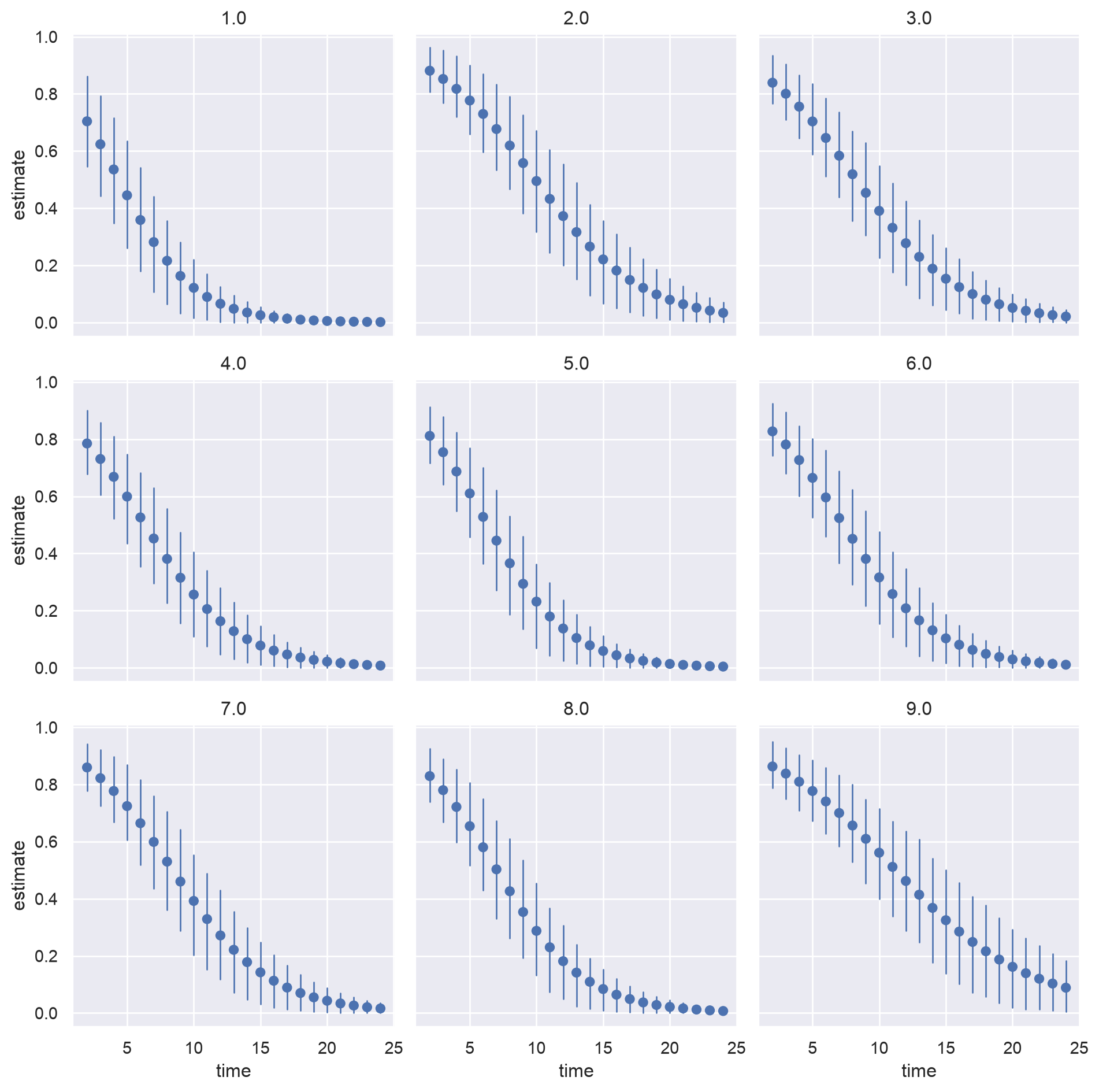
Visualize the model fit for 9 first dogs.

first9 = list(dogs_df["dog"].unique()[:9])

bmb.interpret.plot_predictions(
    model_0h,
    idata_0h,
    conditional={"time": None, "dog": first9},
    subplot_kwargs={"main": "time", "panel": "dog"},
    fig_kwargs={"theme": {"figure.figsize": (10, 10)}, "wrap": 3},
)

4.3 Predictive calibration check

Examine how well the leave-one-out predictive probabilities are calibrated using PAV-adjusted calibration plot. Looks quite good.

az.plot_loo_pava(idata_0h);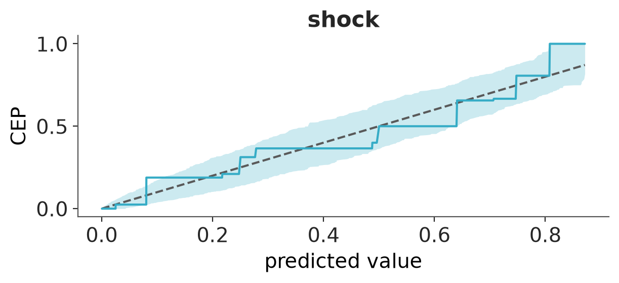

Figure 1

4.4 Residual plots

az.plot_ppc_pava_residuals(idata_0h, x_var=dogs_df["time"])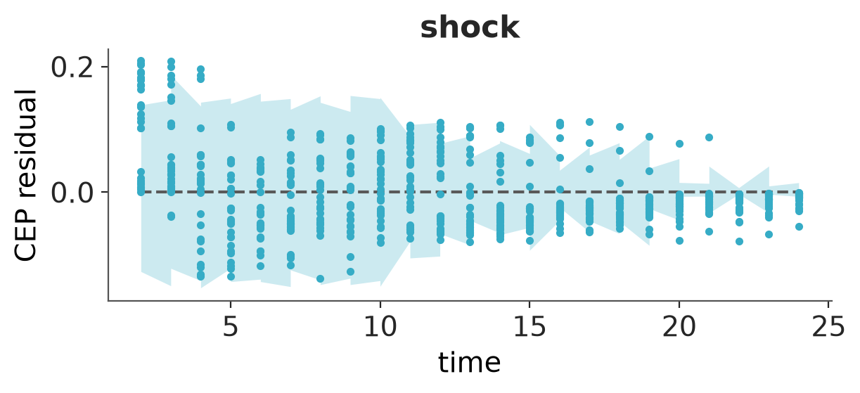

Figure 2

4.5 Posterior predictive checking

Visual posterior predictive checking plotting predicted shocks and avoidances by ordering the dogs with last observed shock.

def plot_ppc_shocks(ax, y, title=""):
    J, T = y.shape
    max_y_times = np.full(J, -1)
    for j in range(J):
        shock_times = np.where(y[j] == 1)[0]
        if len(shock_times) > 0:
            max_y_times[j] = shock_times.max()
    order = np.argsort(max_y_times)[::-1]
    y_ordered = y[order]
    ax.imshow(y_ordered, aspect="auto", cmap=shock_cmap, origin="lower",
              interpolation="nearest")
    ax.set(xticks=[], yticks=[], title=title)

pp_samples_0h = az.extract(idata_0h, group="posterior_predictive",
                            num_samples=1, random_seed=SEED)
y_rep_0h = pp_samples_0h.values.reshape(n_dogs, n_trials-1)

fig, (ax1, ax2) = plt.subplots(1, 2, figsize=(8, 3))
plot_ppc_shocks(ax1, shock_matrix, "Real dogs")
plot_ppc_shocks(ax2, y_rep_0h, "Model 0h: hier. logit")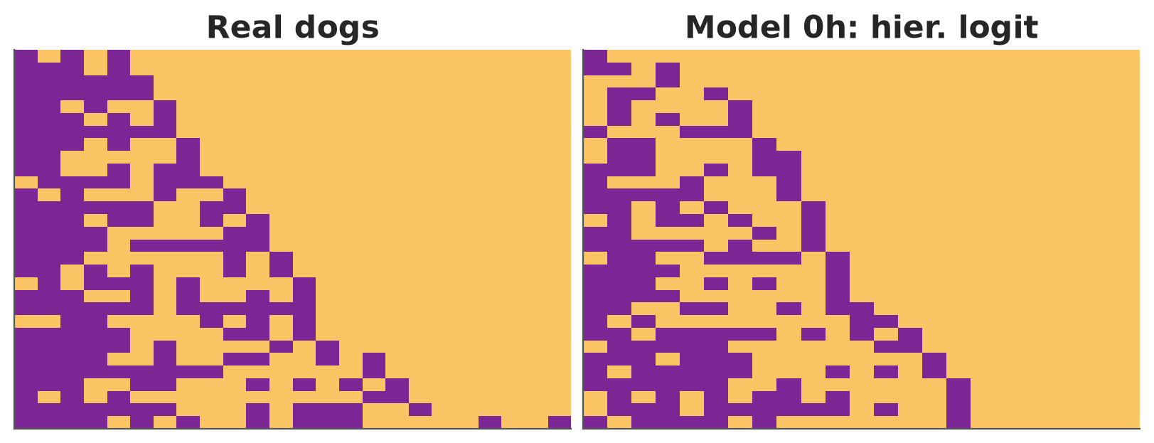

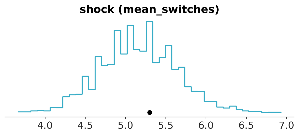
Figure 3

Posterior predictive checking using mean number of switches between shocks and avoidances as the test statistic.

def mean_switches(x):
    x = x.reshape(n_dogs, n_trials-1)
    return np.mean(np.sum(np.abs(np.diff(x, axis=1)), axis=1))

az.plot_ppc_tstat(
    idata_0h,
    t_stat=mean_switches,
    kind="hist",
)

4.6 Prior-likelihood sensitivity analysis

Using powerscaling prior-likelihood sensitivity analysis (Kallioinen et al. 2023) shows that the data are informative and there is no need to think more about priors unless we do happen to have easily available strong prior information.

az.psense_summary(idata_0h, var_names=["~p", "~time|dog", "~1|dog"])

	prior	likelihood	diagnosis
Intercept	0.019	0.156	✓
time	0.017	0.175	✓
1|dog_sigma	0.007	0.240	✓
time|dog_sigma	0.009	0.242	✓

5 Model 1: 1-parameter log model

Coming soon:

References

Bush, R. R., and F. Mosteller. 1955. Stochastic Models for Learning. Wiley.

Kallioinen, Noa, Topi Paananen, Paul-Christian Bürkner, and Aki Vehtari. 2023. “Detecting and Diagnosing Prior and Likelihood Sensitivity with Power-Scaling.” Statistics and Computing 34 (1): 57.

Vehtari, Aki, Andrew Gelman, and Jonah Gabry. 2017. “Practical Bayesian Model Evaluation Using Leave-One-Out Cross-Validation and WAIC.” Statistics and Computing 27: 1413–32.