---
title: "Model building and expansion for golf putting"
image: ../social_cards/golf.png
author: "Andrew Gelman and Aki Vehtari"
date: 2019-09-24
date-modified: today
date-format: iso
format:
html:
number-sections: true
code-copy: true
code-download: true
code-tools: true
bibliography: ../casestudies.bib
---
This notebook includes the code for Bayesian Workflow book chapter
25 *Model building and expansion: Golf putting*.
## Introduction
We demonstrate the basic workflow of Bayesian modeling using an
example of a set of models fit to data on golf putting.
```{python}
#| label: setup
#| include: true
#| cache: false
import sys
import warnings
sys.path.insert(0, '..')

import arviz as az
import matplotlib.pyplot as plt
import numpy as np
import pandas as pd
import xarray as xr
from scipy.special import expit
import preliz as pz
from cmdstanpy import CmdStanModel, disable_logging

from utils import print_stan

warnings.filterwarnings("ignore")
disable_logging()

az.style.use("arviz-variat")
az.rcParams["stats.ci_prob"] = 0.95
plt.rcParams["figure.dpi"] = 100
SEED = 7412
```
```{python}
# utility function for plotting the data
def plot_common(title, plot_observations=True):
    _, ax = plt.subplots(figsize=(10, 5))
    if plot_observations:
        ax.scatter(x, y / n, color="k")
        ax.errorbar(x, y / n, yerr=se, fmt="none", color="k")

    ax.set(xlim=(0, x.max() + 1),
        ylim=(0, 1.02),
        xlabel="Distance from hole (feet)",
        ylabel="Probability of success",
        title=title)
    return ax

# utility function to convert CmdStanMCMC or CmdStanPathfinder to a list of init dicts for sample()
def cmdstan_inits(fit, chains=4):
    vars_ = list(fit.stan_variables().keys())
    n = len(fit.draws())
    return [
        {var: fit.stan_variable(var)[i % n] for var in vars_}
        for i in range(chains)
    ]
```
## Data
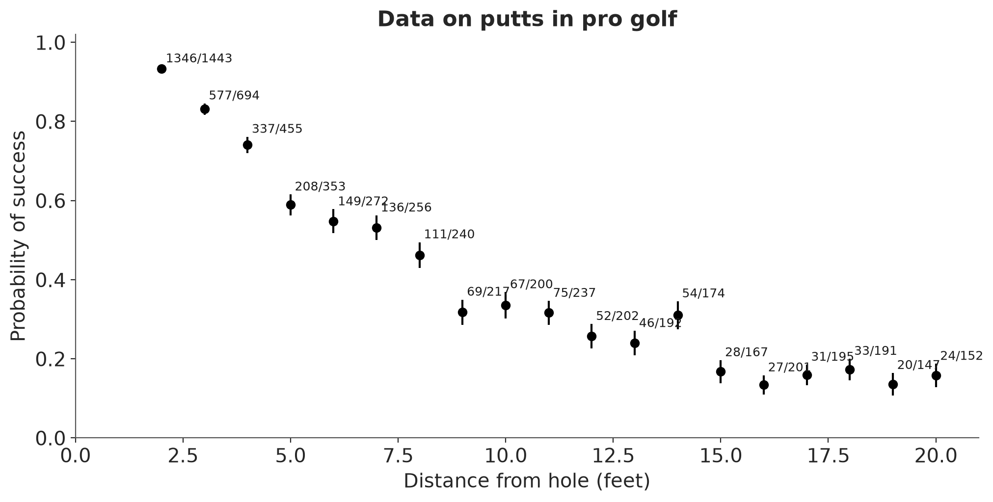
The following graph shows data from professional golfers on the proportion of successful
putts as a function of distance from the hole [from @Berry:1995]. Unsurprisingly, the
probability of making the shot declines as a function of distance:
```{python}
golf = pd.read_csv("data/golf_data.txt", sep=r"\s+", skiprows=2)
x = golf["x"].values
y = golf["y"].values
n = golf["n"].values
J = len(y)
r = (1.68 / 2) / 12
R = (4.25 / 2) / 12
se = np.sqrt((y / n) * (1 - y / n) / n)
```
```{python}
#| label: fig-golf-data
ax = plot_common("Data on putts in pro golf")
for i in range(J):
    ax.annotate(f"{y[i]}/{n[i]}", (x[i] + 0.1, y[i] / n[i] + se[i] + 0.01), fontsize=9, color="0.1")
```
The error bars associated with each point $j$ in the above graph are simple classical standard deviations,
$\sqrt{\hat{p}_j(1-\hat{p}_j)/n_j}$, where $\hat{p}_j=y_j/n_j$ is the success rate for putts taken at distance $x_j$.
## Logistic regression
Can we model the probability of success in golf putting as a function
of distance from the hole? Given usual statistical practice, the
natural starting point would be logistic regression:
$$
y_j\sim\mathrm{binomial}(n_j, \mathrm{logit}^{-1}(a + bx_j)),
\text{ for } j=1,\dots, J.
$$
In Stan, this is:
```{python}
model_1 = CmdStanModel(stan_file=str("golf_logistic.stan"))
print_stan(model_1)
```
The code in the above model block is (implicitly) vectorized, so
that it is mathematically equivalent to modeling each data point,
`y[i] ~ binomial_logit(n[i], a + b*x[i])`. The vectorized code is
more compact (no need to write a loop, or to include the
subscripts) and faster (because of more efficient gradient
evaluations).
We fit the model to the data:
```{python}
#| label: golf_logistic.stan
#| results: hide
golf_data = {"x": x, "y": y, "n": n, "J": J}
fit_1 = model_1.sample(data=golf_data, seed=SEED, show_progress=False)
```
And here is the result:
```{python}
dt_1 = az.from_cmdstanpy(fit_1)
n_sims = dt_1.posterior.sizes["draw"] * dt_1.posterior.sizes["chain"]
df = az.summary(dt_1)
df
```
Going through the columns of the above Table: ArviZ has computed the posterior means $\pm$ standard deviations of $a$ and $b$ to be
`{python} f"{df["mean"].a}"` $\pm$ `{python} f"{df["sd"].a}"` and `{python} f"{df["mean"].b}"` $\pm$ `{python} f"{df["sd"].b}"`, respectively. The Monte Carlo standard error of the mean of each of these parameters is 0 (to two decimal places), indicating that the simulations have run long enough to estimate the posterior means precisely. The posterior quantiles give a sense of the uncertainty
in the parameters, with 50% posterior intervals of
[`{python} f"{np.quantile(dt_1.posterior.a.values, 0.25):.2f}"`,
`{python} f"{np.quantile(dt_1.posterior.a.values, 0.75):.2f}"`] and
[`{python} f"{np.quantile(dt_1.posterior.b.values, 0.25):.2f}"`,
`{python} f"{np.quantile(dt_1.posterior.b.values, 0.75):.2f}"`] for $a$ and $b$, respectively.
Finally, the values of $\widehat{R}$ near 1 tell us that the
four simulated chains have mixed well.
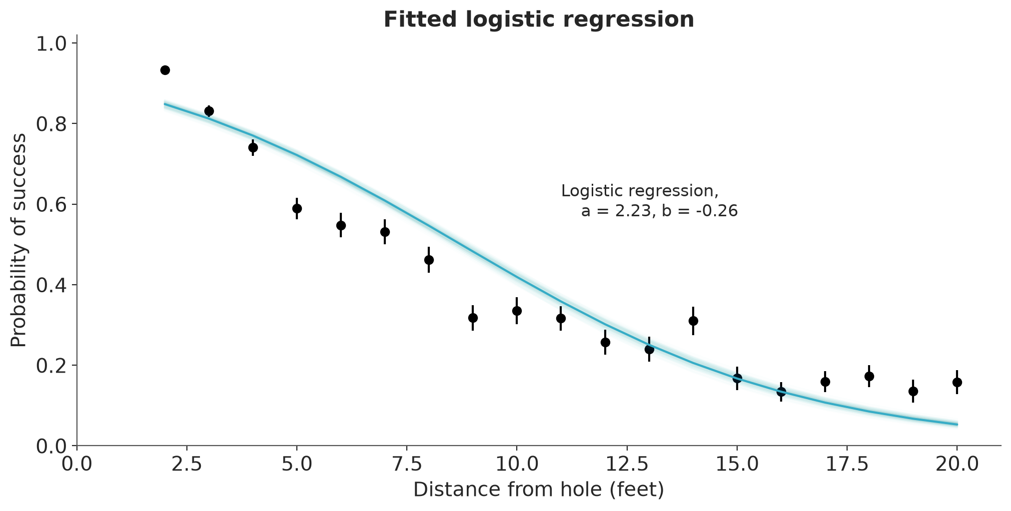
The following graph shows the fit plotted along with the data:
```{python}
#| label: fig-golf-fit1
post_rng = az.extract(dt_1, num_samples=100, random_seed=SEED)
hats = az.mean(dt_1, round_to="None")

x_da = xr.DataArray(x, dims=["x"])
y_pred_lr = expit(post_rng["a"] + post_rng["b"] * x_da).T
y_pred_lr_mean = expit(hats["a"] + hats["b"] * x_da)

ax = plot_common("Fitted logistic regression")
ax.plot(x_da, y_pred_lr, color="C0", alpha=0.01)
ax.plot(x_da, y_pred_lr_mean, color="C0")
ax.annotate(f"Logistic regression,\n    a = {hats["a"]:.2f}, b = {hats["b"]:.2f}", xy=(11, 0.57))
```
The black line shows the fit corresponding to the posterior median
estimates of the parameters $a$ and $b$; the green lines show 10 draws
from the posterior distribution.
In this example, posterior uncertainties in the fits are small, and
for simplicity we will just plot point estimates based on posterior
median parameter estimates for the remaining models. Our focus
here is on the sequence of models that we fit, not so much on
uncertainty in particular model fits.
## Modeling from first principles
As an alternative to logistic regression, we shall build a model from
first principles and fit it to the data.
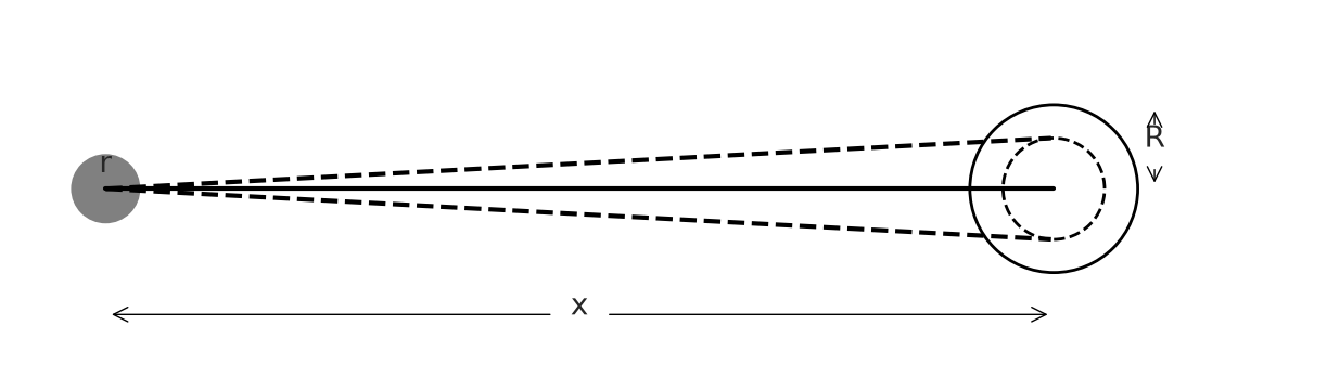
The graph below shows a simplified sketch of a golf shot. The
dotted line represents the angle within which the ball of radius
$r$ must be hit so that it falls within the hole of radius $R$.
This threshold angle is $\sin^{-1}((R-r)/x)$. The graph, which is
not to scale, is intended to illustrate the geometry of the ball
needing to go into the hole.
```{python}
dist = 2
r_plot = r
R_plot = R

_, ax = plt.subplots()
ax.set(xlim=(-R_plot, dist + 3 * R_plot),
       ylim=(-2 * R_plot, 2 * R_plot),
       aspect="equal",
)
ax.axis("off")

circle_ball = plt.Circle((0, 0), r_plot, fill=True, color="gray")
circle_hole_inner = plt.Circle((dist, 0), R_plot - r_plot, fill=False, linestyle="--")
circle_hole_outer = plt.Circle((dist, 0), R_plot, fill=False)
ax.add_patch(circle_ball)
ax.add_patch(circle_hole_inner)
ax.add_patch(circle_hole_outer)

ax.plot([0, dist], [0, 0], "k-")
inner_r = R_plot - r_plot
alpha = np.arcsin(inner_r / dist)
x_tang = dist * np.cos(alpha)**2
y_tang = dist * np.cos(alpha) * np.sin(alpha)

ax.plot([0, x_tang], [0,  y_tang], "k--")
ax.plot([0, x_tang], [0, -y_tang], "k--")

ax.annotate("x", xy=(0.5 * dist, -1.5 * R_plot), fontsize=10, ha="center")
ax.annotate("", xy=(dist, -1.5 * R_plot), xytext=(0.5 * dist + 0.05, -1.5 * R_plot),
            arrowprops=dict(arrowstyle="->", lw=0.5))
ax.annotate("", xy=(0, -1.5 * R_plot), xytext=(0.5 * dist - 0.05, -1.5 * R_plot),
            arrowprops=dict(arrowstyle="->", lw=0.5))

ax.annotate("R", xy=(dist + 1.2 * R_plot, 0.5 * R_plot), fontsize=10, ha="center")
ax.annotate("", xy=(dist + 1.2 * R_plot, R_plot), xytext=(dist + 1.2 * R_plot, 0.7 * R_plot),
            arrowprops=dict(arrowstyle="->", lw=0.5))
ax.annotate("", xy=(dist + 1.2 * R_plot, 0), xytext=(dist + 1.2 * R_plot, 0.3 * R_plot),
            arrowprops=dict(arrowstyle="->", lw=0.5))

ax.annotate("r", xy=(0, r_plot / 2), fontsize=10, ha="center")
```
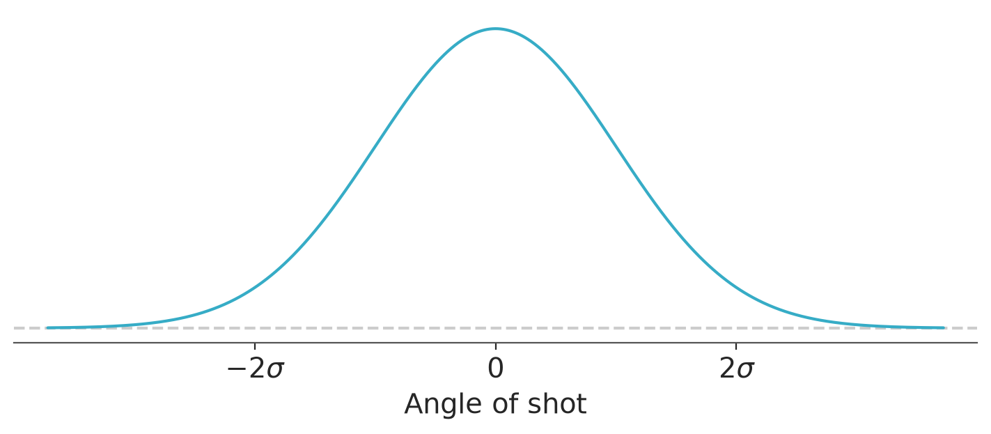
The next step is to model human error. We assume that the golfer is
attempting to hit the ball completely straight but that many small
factors interfere with this goal, so that the actual angle follows a normal distribution centered at 0 with some standard deviation $\sigma$.
```{python}
#| label: fig-golf-sketch-2
ax = pz.Normal(0, 1).plot_pdf(legend=False, figsize=(7, 3))
ax.set(xlim=(-4, 4),
       xlabel="Angle of shot",
       xticks=[-2, 0, 2],
       xticklabels=[r"$-2\sigma$", "0", r"$2\sigma$"],
)
ax.spines[["left"]].set_visible(False);
```
The probability the ball goes in the hole is then the probability
that the angle is less than the threshold; that is,
$\mathrm{Pr}\left(|\mathrm{angle}| < \sin^{-1}((R-r)/x)\right) =
2\Phi\left(\frac{\sin^{-1}((R-r)/x)}{\sigma}\right) - 1$, where
$\Phi$ is the cumulative normal distribution function. The only
unknown parameter in this model is $\sigma$, the standard deviation
of the distribution of shot angles. Stan (and, for that matter, R)
computes trigonometry using angles in radians, so at the end of our
calculations we will need to multiply by $180/\pi$ to convert to
degrees, which are more interpretable by humans.
Our model then has two parts:
\begin{align}
y_j &\sim \mathrm{binomial}(n_j, p_j)\\
p_j &= 2\Phi\left(\frac{\sin^{-1}((R-r)/x_j)}{\sigma}\right) - 1 , \text{ for } j=1,\dots, J.
\end{align}
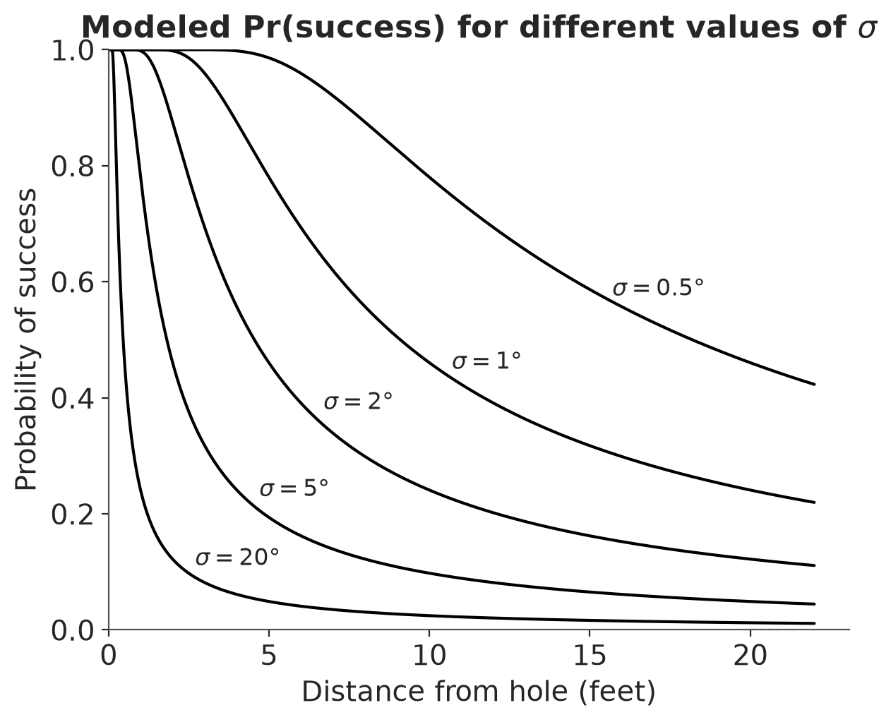
Here is a graph showing the curve for some potential values of the parameter $\sigma$.
```{python}
#| label: fig-golf-angle-curves
fig, ax = plt.subplots()
sigma_degrees_plot = [0.5, 1, 2, 5, 20]
x_text = [15, 10, 6, 4, 2]

for i, sigma_deg in enumerate(sigma_degrees_plot):
    sigma = (np.pi / 180) * sigma_deg
    x_grid = np.arange(R - r, 1.1 * max(x), 0.01)
    p_grid = 2 * pz.Normal(0, 1).cdf(np.arcsin((R - r) / x_grid) / sigma) - 1
    ax.plot(
        np.concatenate([[0, R - r], x_grid]),
        np.concatenate([[1, 1], p_grid]),
        color="black"
    )
    ax.text(
        x_text[i] + 0.7,
        2 * pz.Normal(0, 1).cdf(np.arcsin((R - r) / x_text[i]) / sigma) - 1,
        rf"$\sigma = {sigma_deg}°$",
        va="center"
    )

ax.set(xlim=(0, None),
       ylim=(0, 1),
       xlabel="Distance from hole (feet)",
       ylabel="Probability of success",
       title=r"Modeled Pr(success) for different values of $\sigma$",
);
```
The highest curve on the graph corresponds to $\sigma=0.5^\circ$:
if golfers could control the angles of their putts to an accuracy
of approximately half a degree, they would have a very high
probability of success, making over 80\% of their ten-foot putts,
over 50\% of their fifteen-foot putts, and so on. At the other
extreme, the lowest plotted curve corresponds to $\sigma=20^\circ$:
if your putts could be off as high as 20 degrees, then you would be
highly inaccurate, missing more than half of your two-foot
putts. When fitting the model in Stan, the program moves around the
space of $\sigma$, sampling from the posterior distribution.
We now write the Stan model in preparation to estimating $\sigma$:
```{python}
model_2 = CmdStanModel(stan_file=str("golf_angle_binomial.stan"))
print_stan(model_2)
```
In the transformed data block above, the `./` in the calculation of p corresponds to componentwise division in this vectorized
computation.
The data $J,n,x,y$ have already been set up; we just need to define $r$ and $R$ (the golf ball and hole have diameters 1.68 and 4.25 inches, respectively), and run the Stan model:
```{python}
#| label: golf_angle_binomial.stan
#| results: hide
golf_data = {**golf_data, "r": r, "R": R}
fit_2 = model_2.sample(data=golf_data, seed=SEED, show_progress=False)
```
Here is the result:
```{python}
dt_2 = az.from_cmdstanpy(fit_2)
df = az.summary(dt_2)
df
```
The model has a single parameter, $\sigma$. From the output, we
find that Stan has computed the posterior mean of $\sigma$ to be
`{python} f"{df["mean"]["sigma"]}"`. Multiplying this by $180/\pi$,
this comes to `{python} f"{df["mean"]["sigma_degrees"]}"` degrees.
The Monte Carlo standard error of the mean is 0 (to two decimal
places), indicating that the simulations have run long enough to
estimate the posterior mean precisely. The posterior standard
deviation is calculated at `{python} f"{df["sd"]["sigma_degrees"]}"`
degrees, indicating that $\sigma$ itself
has been estimated with high precision, which makes sense given the
large number of data points and the simplicity of the model. The
precise posterior distribution of $\sigma$ can also be seen from
the narrow range of the posterior quantiles. Finally,
$\widehat{R}$ is near 1, telling us that the simulations from
Stan's four simulated chains have mixed well.
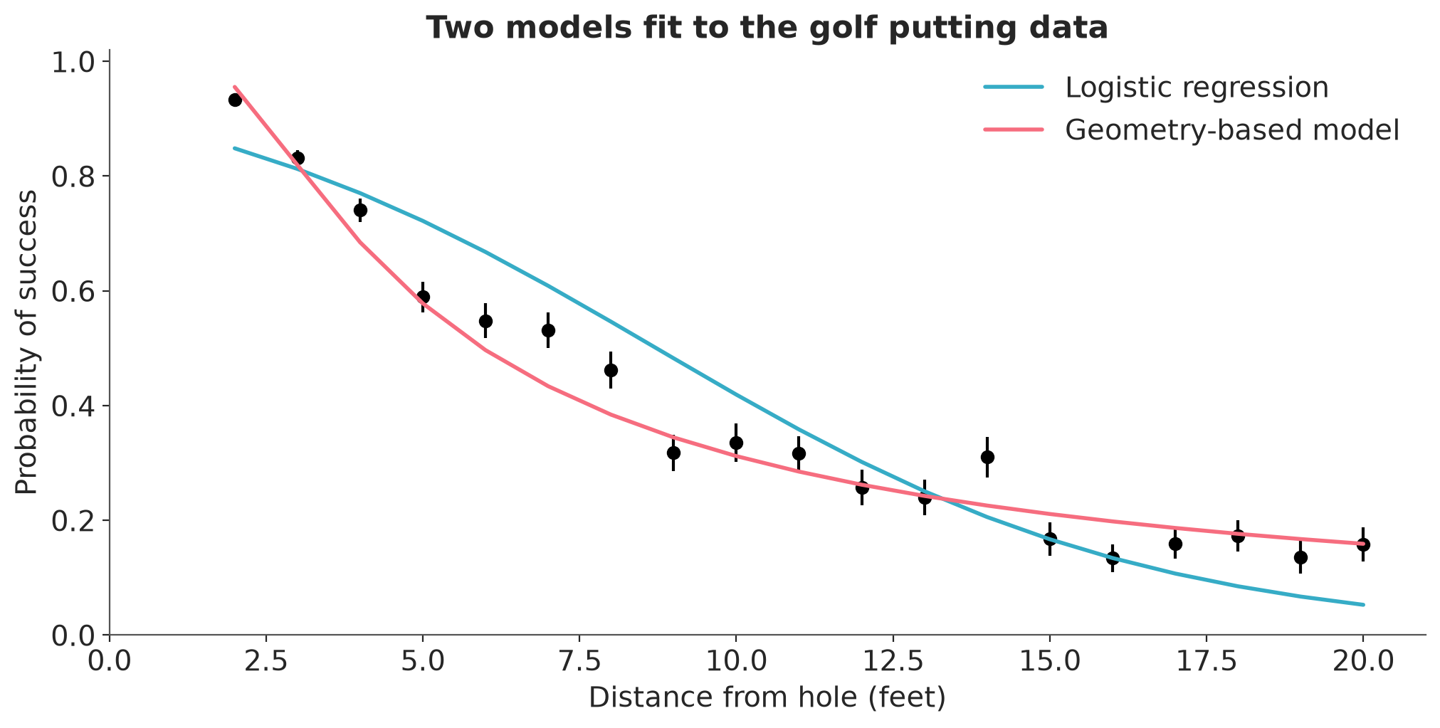
We next plot the data and the fitted model (here using the
posterior median of $\sigma$ but in this case the uncertainty is so narrow that any reasonable posterior summary would give essentially the same result), along with the logistic regression fitted earlier:
```{python}
#| label: fig-golf-fit-1-2
hats = az.mean(dt_2, round_to="None")
sigma_hat = hats["sigma"].item()
y_pred_gb_mean = 2 * pz.Normal(0, 1).cdf(np.arcsin((R - r) / x_da) / sigma_hat) - 1

ax = plot_common("Two models fit to the golf putting data")
ax.plot(x_da, y_pred_lr_mean, color="C0", label="Logistic regression", lw=2)

ax.plot(x_da, y_pred_gb_mean, color="C1", label="Geometry-based model", lw=2)

plt.legend()
```
The custom nonlinear model fits the data much better. This is not to say that the model is perfect---any experience of golf will reveal that the angle is not the only factor determining whether the ball goes in the hole---but it seems like a useful start.
## Testing the fitted model on new data
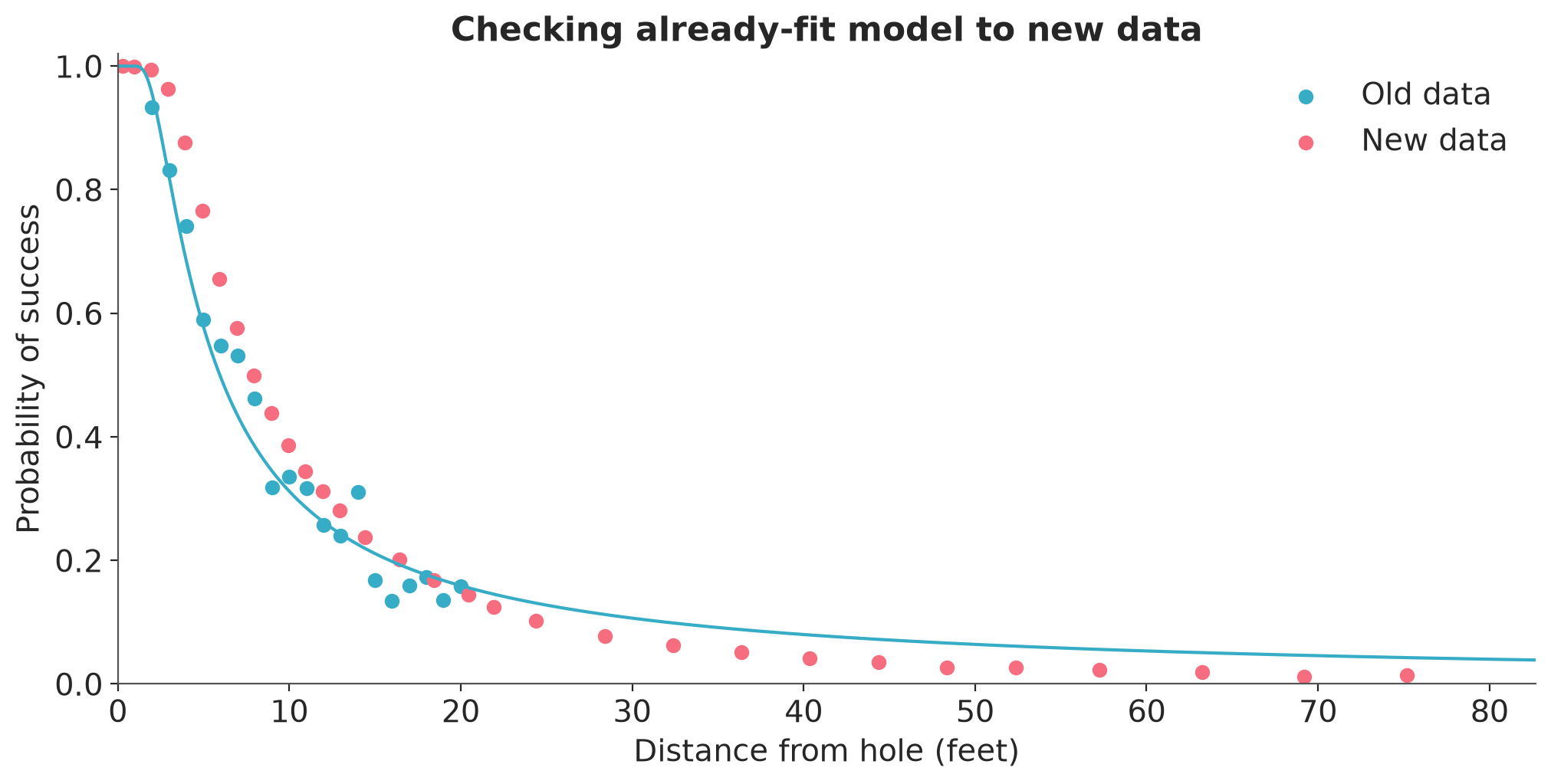
Several years after fitting the above model, we were presented with a newer and more comprehensive dataset on professional golf putting [@Broadie:2018]. For simplicity we'll just look here at the summary data, probabilities of the ball going into the hole for shots up to 75 feet from the hole. The graph below shows these new data (in red), along with our earlier dataset (in blue) and the already-fit geometry-based model from before, extending to the range of the new data.
```{python}
golf_new = pd.read_csv("data/golf_data_new.txt", sep=r"\s+", skiprows=2)
```
```{python}
#| label: fig-golf-fit-2-new
ax = plot_common(title="Checking already-fit model to new data", plot_observations=False)
x_grid = np.arange(R - r, 1.1 * golf_new["x"].max(), 0.01)
p_grid = 2 * pz.Normal(0, 1).cdf(np.arcsin((R - r) / x_grid) / sigma_hat) - 1
ax.plot(np.concatenate([[0, R - r], x_grid]),
        np.concatenate([[1, 1], p_grid]), color="C0")
ax.scatter(golf["x"], golf["y"] / golf["n"], color="C0", label="Old data")
ax.scatter(golf_new["x"], golf_new["y"] / golf_new["n"], color="C1", label="New data")
ax.set_xlim(0, 1.1 * golf_new["x"].max())
ax.legend()
```
Comparing the two datasets in the range 0-20 feet, the success rate is similar for longer putts but is much higher than before for the short putts. This could be a measurement issue, if the distances to the hole are only approximate for the old data, and it could also
be that golfers are better than they used to be.
Beyond 20 feet, the empirical success rates become lower than would be predicted by the old model. These are much more difficult attempts, even after accounting for the increased angular precision required as distance goes up. In addition, the new data look smoother, which perhaps is a reflection of more comprehensive data collection.
## A new model accounting for how hard the ball is hit
To get the ball in the hole, the angle isn't the only thing you
need to control; you also need to hit the ball just hard enough.
@Broadie:2018 added this feature to the geometric model by
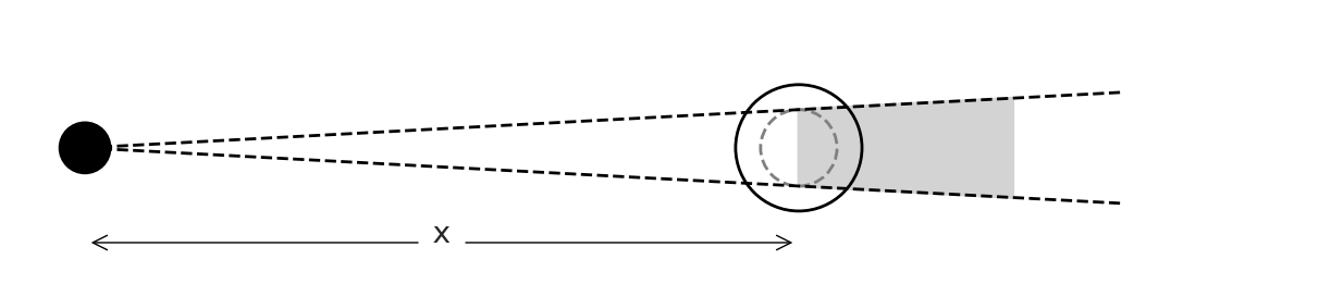
introducing another parameter corresponding to the golfer's control over distance. Supposing $u$ is the distance that golfer's shot would travel if there were no hole, the assumption is that the putt will go in if (a) the angle allows the ball to go over the hole, and (b) $u$ is in the range $(x,x+3)$. That is the ball must be hit just hard enough to reach the hole but not go too far. Factor (a) is what we have considered earlier; we must now add factor (b).
The following sketch, which is not to scale, illustrates the need
for the distance as angle as well as the angle of the shot to be in some range, in this case the gray zone which represents the
trajectories for which the ball would reach the hole and stay in
it.
```{python}
#| label: fig-golf-sketch-3
dist = 2
r_plot = r
R_plot = R
distance_tolerance = 0.6
fig, ax = plt.subplots()
ax.set_xlim(-R_plot, dist + 3 * R_plot + 1.5 * distance_tolerance)
ax.set_ylim(-2 * R_plot, 2 * R_plot)
ax.set_aspect("equal")
ax.axis("off")
polygon_x = [dist, dist, dist + distance_tolerance, dist + distance_tolerance]
polygon_y = [R_plot - r_plot, -(R_plot - r_plot),
             -(R_plot - r_plot) * (dist + distance_tolerance) / dist,
             (R_plot - r_plot) * (dist + distance_tolerance) / dist]
ax.fill(polygon_x, polygon_y, color="lightgray")
circle_ball = plt.Circle((0, 0), r_plot, fill=True, color="black")
circle_hole = plt.Circle((dist, 0), R_plot, fill=False)
circle_hole_inner = plt.Circle((dist, 0), R_plot - r_plot, fill=False, linestyle="--", color="gray")
ax.add_patch(circle_ball)
ax.add_patch(circle_hole)
ax.add_patch(circle_hole_inner)
ax.plot([0, dist + 1.5 * distance_tolerance],
        [(R_plot - r_plot) / dist * 0, (R_plot - r_plot) / dist * (dist + 1.5 * distance_tolerance)],
        "k--", lw=1)
ax.plot([0, dist + 1.5 * distance_tolerance],
        [-((R_plot - r_plot) / dist) * 0, -((R_plot - r_plot) / dist) * (dist + 1.5 * distance_tolerance)],
        "k--", lw=1)
ax.annotate("x", xy=(0.5 * dist, -1.5 * R_plot), fontsize=10, ha="center")
ax.annotate("", xy=(dist, -1.5 * R_plot), xytext=(0.5 * dist + 0.05, -1.5 * R_plot),
            arrowprops=dict(arrowstyle="->", lw=0.5))
ax.annotate("", xy=(0, -1.5 * R_plot), xytext=(0.5 * dist - 0.05, -1.5 * R_plot),
            arrowprops=dict(arrowstyle="->", lw=0.5))
```
Suppose that a golfer will aim to hit the ball one foot past the
hole but with a multiplicative error in the shot's potential
distance, so that $u=(x+1)(1+\epsilon)$, where the error $\epsilon$
has a normal distribution with mean 0 and standard deviation
$\sigma_{\rm distance}$. In statistics notation, this model is,
$u\sim\normal(x+1,(x+1)\sigma_{\rm distance})$, and the distance is
acceptable if $u\in [x,x+3]$, an event that has probability
$\Phi\left(\frac{2}{(x+1)\sigma_{\rm
distance}}\right)-\Phi\left(\frac{-1}{(x+1)\sigma_{\rm
distance}}\right).$
Putting these together, the probability a shot goes in becomes,
$\left(2\Phi\left(\frac{\sin^{-1}((R-r)/x)}{\sigma_{\rm
angle}}\right) -
1\right)\left(\Phi\left(\frac{2}{(x+1)\,\sigma_{\rm
distance}}\right) - \Phi\left(\frac{-1}{(x+1)\,\sigma_{\rm
distance}}\right)\right)$, where we have renamed the parameter
$\sigma$ from our earlier model to $\sigma_{\rm angle}$ to
distinguish it from the new $\sigma_{\rm distance}$ parameter. We
write the new model in Stan, giving it the name
`golf_angle_distance_binomial.stan` to convey that it accounts both
for angle and distance:
```{python}
model_3 = CmdStanModel(stan_file=str("golf_angle_distance_binomial.stan"))
print_stan(model_3)
```
The result is a model with two parameters, $\sigma_{\rm angle}$ and $\sigma_{\rm distance}$. Even this improved geometry-based model is a gross oversimplification of putting, and the average distances in the binned data are not the exact distances for each shot. But it should be an advance on the earlier one-parameter model; the next step is to see how it fits the data.
Here we have defined `overshot` and `distance_tolerance` as data,
which @Broadie:2018 has specified as 1 and 3 feet, respectively.
We might wonder why if the distance range is 3 feet, the overshot
is not 1.5 feet. One reason could be that it is riskier to hit the
ball too hard than too soft. In addition we assigned weakly
informative half-normal(0,1) priors on the scale parameters,
$\sigma_{\rm angle}$ and $\sigma_{\rm distance}$, which are
required in this case to keep the computations stable.
We fit the model to the new dataset.
```{python}
#| label: golf_angle_distance_binomial.stan
#| results: hide
overshot = 1
distance_tolerance = 3
golf_new_data = {
    "x": golf_new["x"].values.tolist(),
    "y": golf_new["y"].values.tolist(),
    "n": golf_new["n"].values.tolist(),
    "J": len(golf_new),
    "r": r,
    "R": R,
    "overshot": overshot,
    "distance_tolerance": distance_tolerance,
}
fit_3 = model_3.sample(data=golf_new_data, seed=SEED, show_progress=False)
```
Here is the result:
```{python}
dt_3 = az.from_cmdstanpy(fit_3)
az.summary(dt_3)
```
There is poor convergence. Very high Rhat and very low ESSs
indicate multimodality. We try initializing MCMC with Pathfinder
```{python}
#| results: hide
pth_3 = model_3.pathfinder(
    data=golf_new_data,
    num_paths=20,
    max_lbfgs_iters=100
)
fit_3 = model_3.sample(
    data=golf_new_data,
    inits=cmdstan_inits(pth_3),
    show_progress=False
)
```
Here is the result:
```{python}
dt_3 = az.from_cmdstanpy(fit_3)
az.summary(dt_3)
```
Now the convergence looks fine.
We graph the new data and the fitted model:
```{python}
#| label: fig-golf-fit-3
sigma_angle_hat = dt_3.posterior["sigma_angle"].values.flatten().mean()
sigma_distance_hat = dt_3.posterior["sigma_distance"].values.flatten().mean()
ax = plot_common(title="Checking model fit", plot_observations=False)
x_grid = np.arange(R - r, 1.1 * golf_new["x"].max(), 0.01)
p_angle_grid = 2 * pz.Normal(0, 1).cdf(np.arcsin((R - r) / x_grid) / sigma_angle_hat) - 1
p_distance_grid = pz.Normal(0, 1).cdf((distance_tolerance - overshot) / ((x_grid + overshot) * sigma_distance_hat)) - \
    pz.Normal(0, 1).cdf(-overshot / ((x_grid + overshot) * sigma_distance_hat))
p_grid = p_angle_grid * p_distance_grid
ax.plot(np.concatenate([[0, R - r], x_grid]),
        np.concatenate([[1, 1], p_grid]), color="C2")
ax.scatter(golf_new["x"], golf_new["y"] / golf_new["n"], color="C2");
```
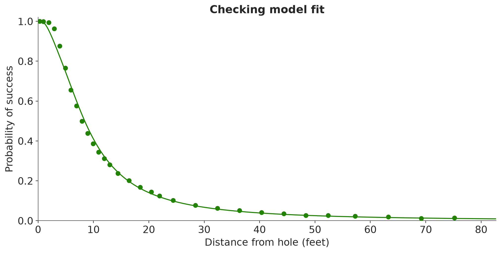
There are problems with the fit in the middle of the range of $x$.
We suspect this is a problem with the binomial error model, as it
tries harder to fit points where the counts are higher. Look at
how closely the fitted curve hugs the data at the very lowest
values of $x$.
Here are the first few rows of the data:
```{python}
golf_new.head()
```
With such large values of $n_j$, the binomial likelihood enforces
an extremely close fit at these first few points, and that drives
the entire fit of the model.
## Expanding the model by including a fudge factor
To fix this problem we took the data model, $y_j \sim
\mathrm{binomial}(n_j, p_j)$, and added an independent error term to each observation. There is no easy way to add error directly to the binomial distribution---we could replace it with its
overdispersed generalization, the beta-binomial, but this would not be appropriate here because the variance for each data point $i$ would still be roughly proportional to the sample size $n_j$, and our whole point here is to get away from this assumption and allow for model misspecification---so instead we first approximate the binomial data distribution by a normal and then add independent variance; thus: $$y_j/n_j \sim \mathrm{normal}\left(p_j, \sqrt{p_j(1-p_j)/n_j + \sigma_y^2}\right),$$ To write this in Stan there are some complications:
* $y$ and $n$ are integer variables, which we convert to vectors so that we can multiply and divide them.
* To perform componentwise multiplication or division using
vectors, you need to use `.*` or `./` so that San knows not to
try to perform vector/matrix multiplication and division. Stan
is opposite from R in this way: Stan defaults to vector/matrix
operations and has to be told otherwise, whereas R defaults to
componentwise operations, and vector/matrix multiplication in R
is indicated using the `%*%` operator.
We implement these via the following new code in the transformed data block:
```stan
vector[J] raw_proportions = to_vector(y) ./ to_vector(n);
```
And then in the model block:
```stan
raw_proportions ~ normal(p, sqrt(p .* (1-p) ./ to_vector(n) + sigma_y^2));
```
To complete the model we add $\sigma_y$ to the parameters block and assign it a weakly informative half-normal(0,1) prior
distribution. Here's the new Stan program:
```{python}
model_4 = CmdStanModel(stan_file=str("golf_angle_distance_normal.stan"))
print_stan(model_4)
```
We now fit this model to the data:
```{python}
#| label: golf_angle_distance_normal.stan
#| results: hide
fit_4 = model_4.sample(data=golf_new_data, seed=SEED, show_progress=False)
```
Here is the result
```{python}
dt_4 = az.from_cmdstanpy(fit_4)
df = az.summary(dt_4)
df
```
The new parameter estimates are:
* $\sigma_{\rm angle}$ is estimated at `{python} f"{df["mean"]["sigma_angle"]}"`, which corresponds to
$\sigma_{\rm degrees}=$ `{python} f"{df["mean"]["sigma_degrees"]}"`. According to the fitted
model, there is a standard deviation of `{python} f"{df["mean"]["sigma_degrees"]}"`
degree in the angles of putts taken by pro golfers. The estimate of $\sigma_{\rm angle}$
has decreased compared to the earlier model that only had angular
errors. This makes sense: now that distance errors have been
included in the model, there is no need to explain so many of the
missed shots using errors in angle.
* $\sigma_{\rm distance}$ is estimated at `{python} f"{df["mean"]["sigma_distance"]}"`. According to the fitted
model, there is a standard deviation of 8\% in the errors of
distance.
* $\sigma_y$ is estimated at `{python} f"{df["mean"]["sigma_y"]}"`. The fitted model fits the
aggregate data (success rate as a function of distance) to an
accuracy of `{python} f"{float(df["mean"]["sigma_y"]) * 100:.1f}"`
percentage points.
And now we graph:
```{python}
#| label: fig-golf-fit-4
hats = az.mean(dt_4, round_to="None")
sigma_angle_hat = hats["sigma_angle"]
sigma_distance_hat = hats["sigma_distance"]
ax = plot_common(title="Checking model fit", plot_observations=False)
x_grid = np.arange(R - r, 1.1 * golf_new["x"].max(), 0.01)
p_angle_grid = 2 * pz.Normal(0, 1).cdf(np.arcsin((R - r) / x_grid) / sigma_angle_hat.item()) - 1
p_distance_grid = pz.Normal(0, 1).cdf((distance_tolerance - overshot) / ((x_grid + overshot) * sigma_distance_hat.item())) - \
    pz.Normal(0, 1).cdf(-overshot / ((x_grid + overshot) * sigma_distance_hat.item()))
p_grid = p_angle_grid * p_distance_grid
ax.plot(np.concatenate([[0, R - r], x_grid]),
        np.concatenate([[1, 1], p_grid]), color="C3")
ax.scatter(golf_new["x"], golf_new["y"] / golf_new["n"], color="C3", zorder=3)
```
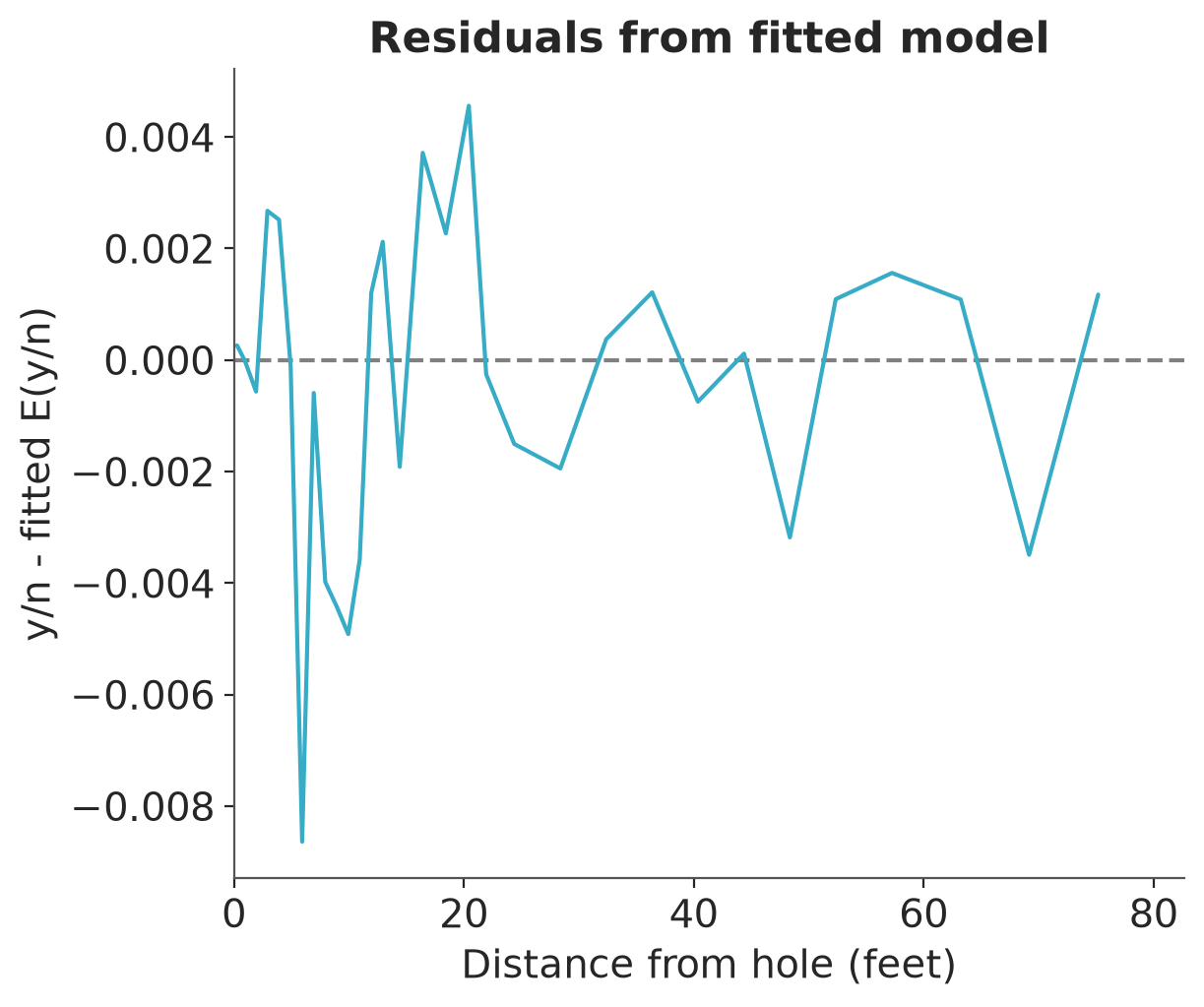
We can go further and plot the residuals from this fit. First we
augment the Stan model to compute residuals in the generated
quantities block.
```{python}
#| label: golf_angle_distance_normal_with_resids.stan
#| results: hide
model_4_with_resids = CmdStanModel(stan_file=str("golf_angle_distance_normal_with_resids.stan"))
fit_4_with_resids = model_4_with_resids.sample(data=golf_new_data, seed=SEED, show_progress=False)
```
Then we compute the posterior means of the residuals, $y_j/n_j -
p_j$, then plot these vs. distance:
```{python}
#| label: fig-golf-res-4
draws_4wr = az.from_cmdstanpy(fit_4_with_resids)
posterior_mean_residual = az.mean(draws_4wr.posterior["residual"])
fig, ax = plt.subplots()
ax.set(xlim=(0, 1.1 * golf_new["x"].max()),
       xlabel="Distance from hole (feet)",
       ylabel="y/n - fitted E(y/n)",
       title="Residuals from fitted model")
ax.axhline(0, color="gray", linestyle="--")
ax.plot(golf_new["x"], posterior_mean_residual)
```
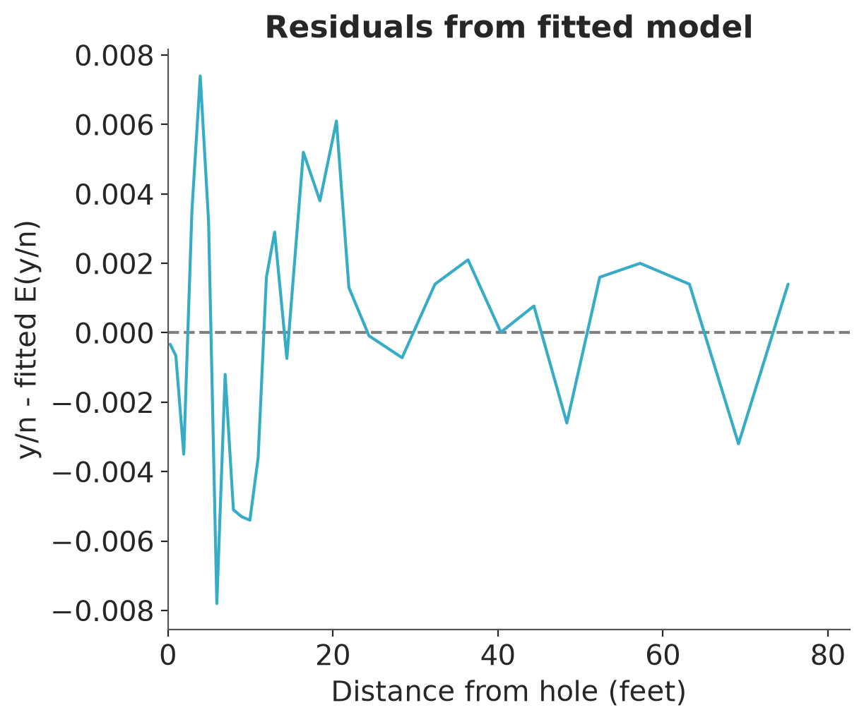
The fit is good, and the residuals show no strong pattern, also
they are low in absolute value---the model predicts the success
rate to within half a percentage point at most distances,
suggesting not that the model is perfect but that there are no
clear problems given the current data.
The above model fit, but we were bothered by the normal
approximation, not so much for these particular data but rather
because it was a sort of admission of failure to not be able to
directly use the binomial model.
## Binomial with errors in logit scale
What we wanted to do was to keep the binomial model and then add
the error on the logistic scale or something like that, something
to keep the probabilities bounded between 0 and 1. We added an
error term on the logistic scale with a scale parameter, `sigma_eta`,
estimated from the data.
```{python}
model_5 = CmdStanModel(stan_file=str("golf_angle_distance_binomial_with_logit_errors.stan"))
print_stan(model_5)
```
We fit the model to the data:
```{python}
#| label: golf_angle_distance_binomial_with_logit_errors.stan
#| results: hide
fit_5 = model_5.sample(data=golf_new_data, seed=SEED, show_progress=False)
```
Here is the result:
```{python}
dt_5 = az.from_cmdstanpy(fit_5)
az.summary(dt_5, var_names=["~eta"])
```
Unfortunately, when we try to fit this new model to our data, the
console fills up with warnings and the chains don't mix. We try
initializing with Pathfinder.
```{python}
#| results: hide
pth_5 = model_5.pathfinder(
    data=golf_new_data,
    num_paths=20,
    max_lbfgs_iters=100
)

fit_5 = model_5.sample(
    data=golf_new_data,
    inits=cmdstan_inits(pth_5),
    show_progress=False
)
```
Here is the result:
```{python}
dt_5 = az.from_cmdstanpy(fit_5)
az.summary(dt_5, var_names=["~eta"])
```
The sampling is slower than for earlier models, but the convergence diagnostic look just fine.
We graph the new data and the fitted model:
```{python}
#| label: fig-golf-fit-5
hats = az.mean(dt_5, round_to="None")

sigma_angle_hat = hats["sigma_angle"].item()
sigma_distance_hat = hats["sigma_distance"].item()
ax = plot_common(title="Checking model fit", plot_observations=False)
ax.set_xlim(0, 1.1 * golf_new["x"].max())
x_grid = np.arange(R - r, 1.1 * golf_new["x"].max(), 0.01)
p_angle_grid = 2 * pz.Normal(0, 1).cdf(np.arcsin((R - r) / x_grid) / sigma_angle_hat) - 1
p_distance_grid = pz.Normal(0, 1).cdf((distance_tolerance - overshot) / ((x_grid + overshot) * sigma_distance_hat)) - \
    pz.Normal(0, 1).cdf(-overshot / ((x_grid + overshot) * sigma_distance_hat))
p_grid = p_angle_grid * p_distance_grid
ax.plot(np.concatenate([[0, R - r], x_grid]),
        np.concatenate([[1, 1], p_grid]), color="C4")
ax.scatter(golf_new["x"], golf_new["y"] / golf_new["n"], color="C4", zorder=3)
```
There are now problems with the fit in the low range of $x$.
Clearly the additive error in logit scale is not good.
## Binomial with proportional errors
Instead of additive errors in logit scale, we next fit a
three-parameter model that scales all the probabilities down from
1. Each observation has its own proportional error term. The key is
to make each element of the multiplier vector `(1- epsilon)`
positive and less than 1. This eliminates the problem with the
boundary and the need for the logit. The prior distribution for
`epsilon` keeps the errors under control.
```{python}
model_6 = CmdStanModel(stan_file=str("golf_angle_distance_binomial_with_proportional_errors.stan"))
print_stan(model_6)
```
We fit the model to the data:
```{python}
#| label: golf_angle_distance_binomial_with_proportional_errors.stan
#| results: hide
fit_6 = model_6.sample(data=golf_new_data, seed=SEED, show_progress=False)
```
Here is the result:
```{python}
dt_6 = az.from_cmdstanpy(fit_6)
az.summary(dt_6, var_names="sigma", filter_vars="like")
```
We graph the new data and the fitted model:
```{python}
#| label: fig-golf-fit-6
hats = az.mean(dt_6, round_to="None")
sigma_angle_hat = hats["sigma_angle"].item()
sigma_distance_hat = hats["sigma_distance"].item()
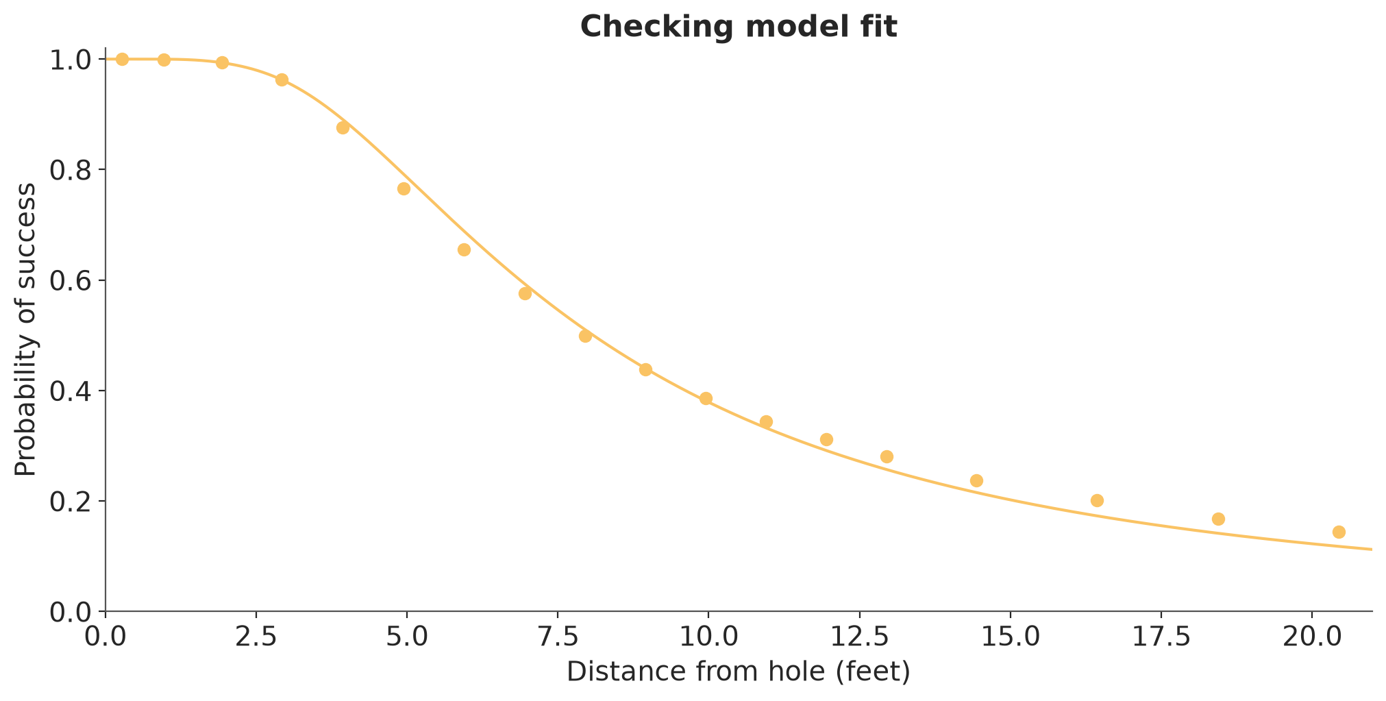
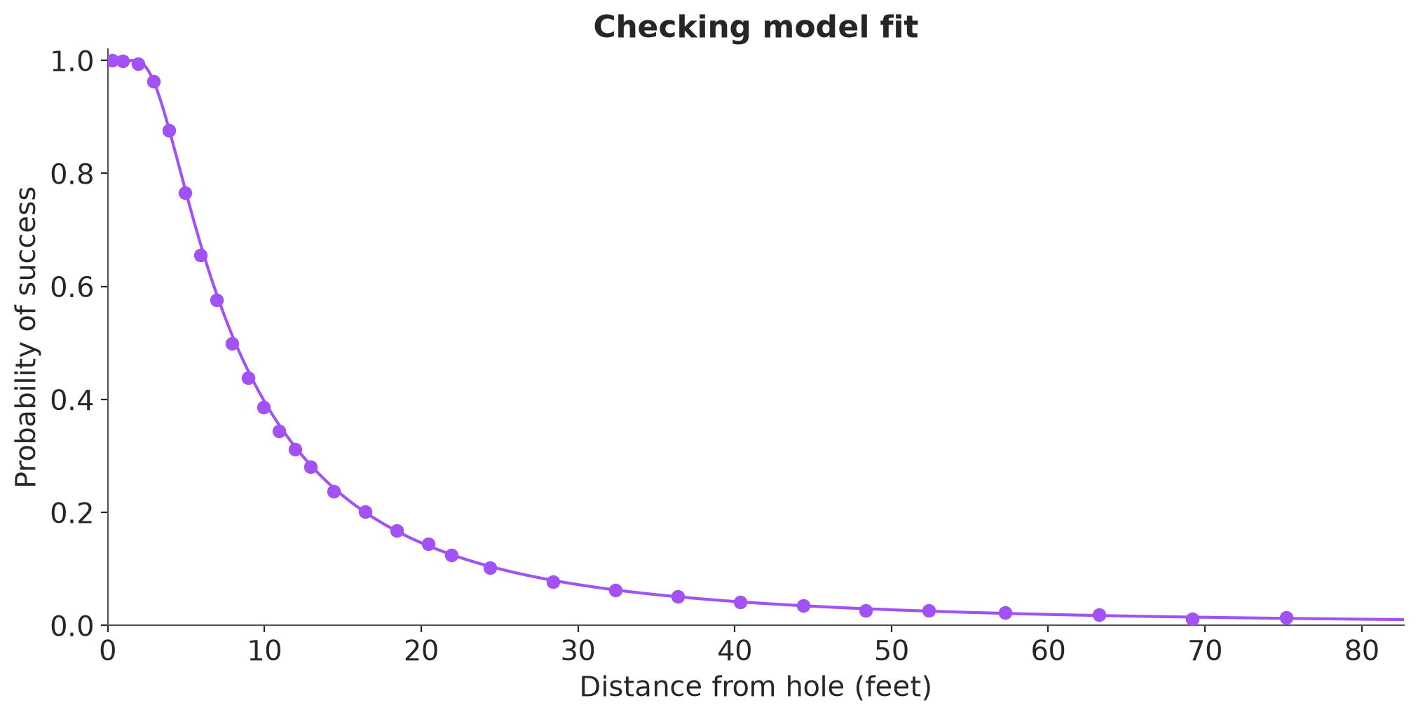
ax = plot_common(title="Checking model fit", plot_observations=False)
ax.set_xlim(0, 1.1 * golf_new["x"].max())
x_grid = np.arange(R - r, 1.1 * golf_new["x"].max(), 0.01)
p_angle_grid = 2 * pz.Normal(0, 1).cdf(np.arcsin((R - r) / x_grid) / sigma_angle_hat) - 1
p_distance_grid = pz.Normal(0, 1).cdf((distance_tolerance - overshot) / ((x_grid + overshot) * sigma_distance_hat)) - \
    pz.Normal(0, 1).cdf(-overshot / ((x_grid + overshot) * sigma_distance_hat))
p_grid = p_angle_grid * p_distance_grid
ax.plot(np.concatenate([[0, R - r], x_grid]),
        np.concatenate([[1, 1], p_grid]), color="C5")
ax.scatter(golf_new["x"], golf_new["y"] / golf_new["n"], color="C5", zorder=3)
```
```{python}
#| label: fig-golf-res-6
posterior_mean_residual_6 = az.mean(dt_6.posterior["residual"],round_to="None")
_, ax = plt.subplots()
ax.set(xlim=(0, 1.1 * golf_new["x"].max()),
       xlabel="Distance from hole (feet)",
       ylabel="y/n - fitted E(y/n)",
       title="Residuals from fitted model")
ax.axhline(0, color="gray", linestyle="--")
ax.plot(golf_new["x"], posterior_mean_residual_6)
```
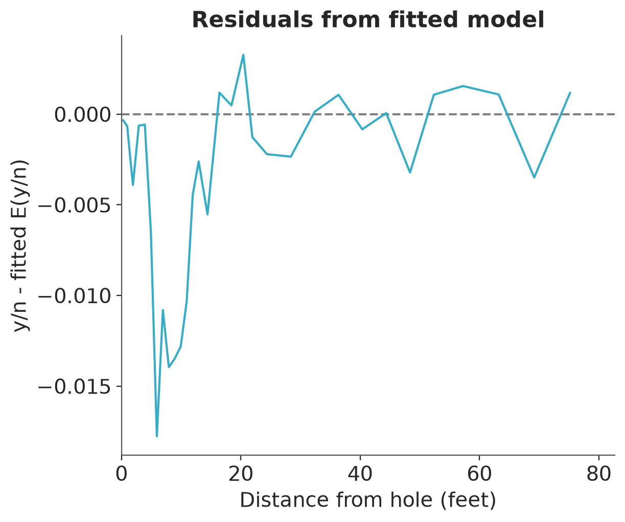
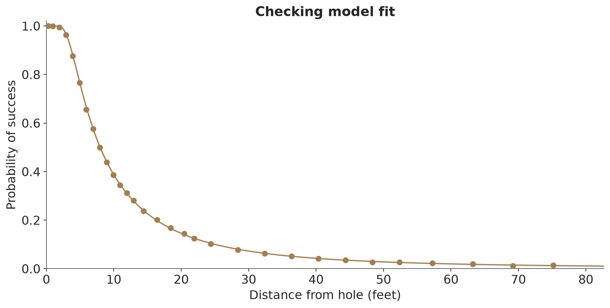
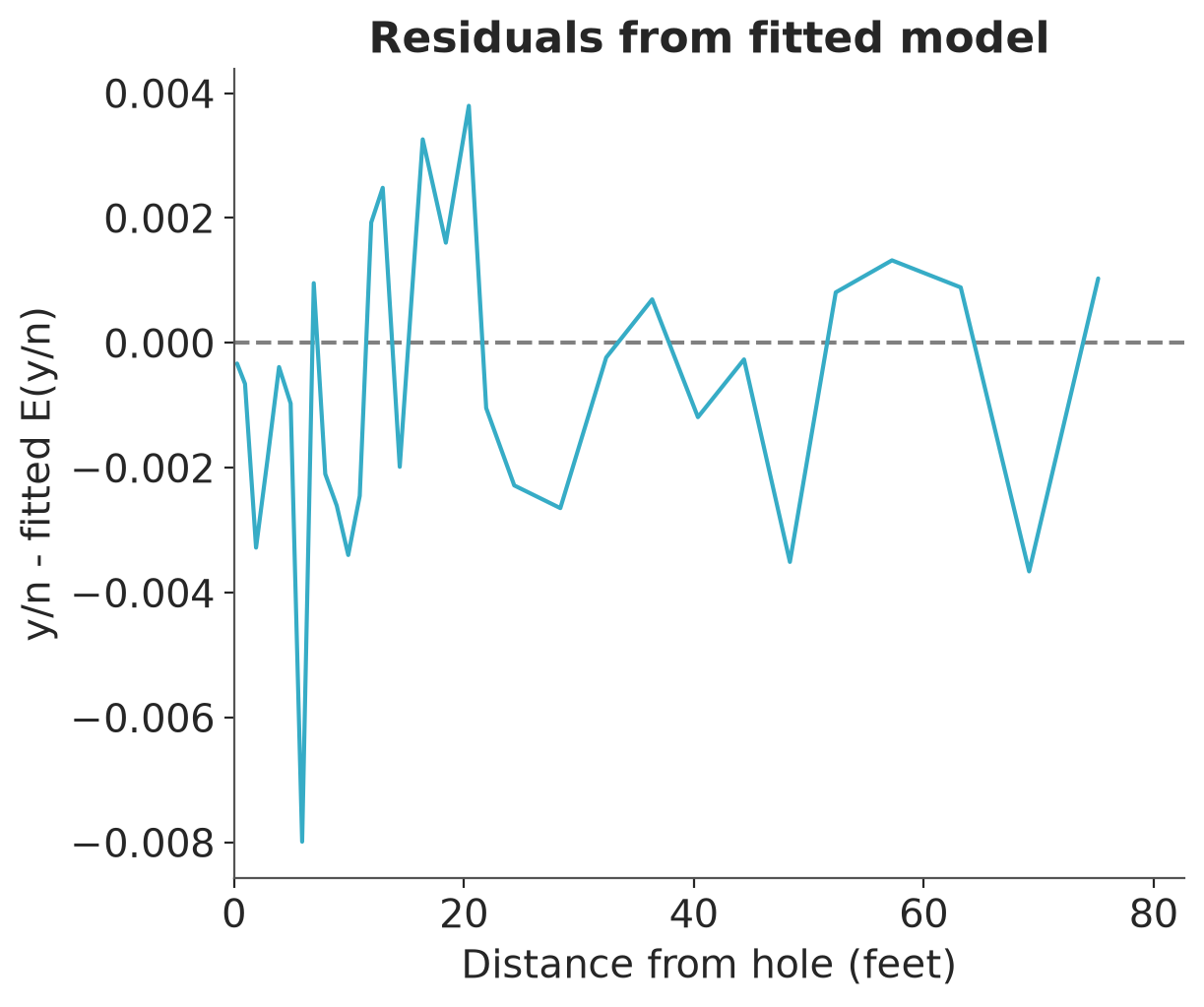
The model fit looks good. The residual plot shows that for short
distances the model overestimates the probabilities. This pattern
could be explained by sensitivity to `distance_tolerance` and
`overshot` parameters that were fixed.
We change `distance_tolerance` to be a parameter. We assume
@Broadie:2018 did use his expertise to choose the value of 3 feet. We use log-normal prior with mean log(3) and standard deviation 0.2 to include that expert information but still have the prior to be relatively weak. We initialize MCMC using the draws from the previous model posterior expect for the new `distance_tolerance` parameter,
```{python}
#| label: golf_angle_distance_binomial_with_proportional_errors_2.stan
#| results: hide
model_7 = CmdStanModel(stan_file="golf_angle_distance_binomial_with_proportional_errors_2.stan")
fit_7 = model_7.sample(data=golf_new_data, seed=SEED, show_progress=False, inits=cmdstan_inits(fit_6))
```
Here is the result:
```{python}
dt_7 = az.from_cmdstanpy(fit_7)
az.summary(dt_7, var_names="sigma", filter_vars="like")
```
We graph the new data and the fitted model:
```{python}
#| label: fig-golf-fit-7
hats = az.mean(dt_7, round_to="None")
sigma_angle_hat = hats["sigma_angle"].item()
sigma_distance_hat = hats["sigma_distance"].item()
distance_tolerance_7 = hats["distance_tolerance"].item()
overshot_7 = 1
ax = plot_common(title="Checking model fit", plot_observations=False)
ax.set_xlim(0, 1.1 * golf_new["x"].max())
x_grid = np.arange(R - r, 1.1 * golf_new["x"].max(), 0.01)
p_angle_grid = 2 * pz.Normal(0, 1).cdf(np.arcsin((R - r) / x_grid) / sigma_angle_hat) - 1
p_distance_grid = pz.Normal(0, 1).cdf((distance_tolerance_7 - overshot_7) / ((x_grid + overshot_7) * sigma_distance_hat)) - \
    pz.Normal(0, 1).cdf(-overshot_7 / ((x_grid + overshot_7) * sigma_distance_hat))
p_grid = p_angle_grid * p_distance_grid
ax.plot(np.concatenate([[0, R - r], x_grid]),
        np.concatenate([[1, 1], p_grid]), color="C6")
ax.scatter(golf_new["x"], golf_new["y"] / golf_new["n"], color="C6", zorder=3)
```
```{python}
#| label: fig-golf-res-7
posterior_mean_residual_7 = az.mean(dt_7.posterior["residual"], round_to="None")
_, ax = plt.subplots()
ax.set_xlim(0, 1.1 * golf_new["x"].max())
ax.set_xlabel("Distance from hole (feet)")
ax.set_ylabel("y/n - fitted E(y/n)")
ax.set_title("Residuals from fitted model")
ax.axhline(0, color="gray", linestyle="--")
ax.plot(golf_new["x"], posterior_mean_residual_7);
```
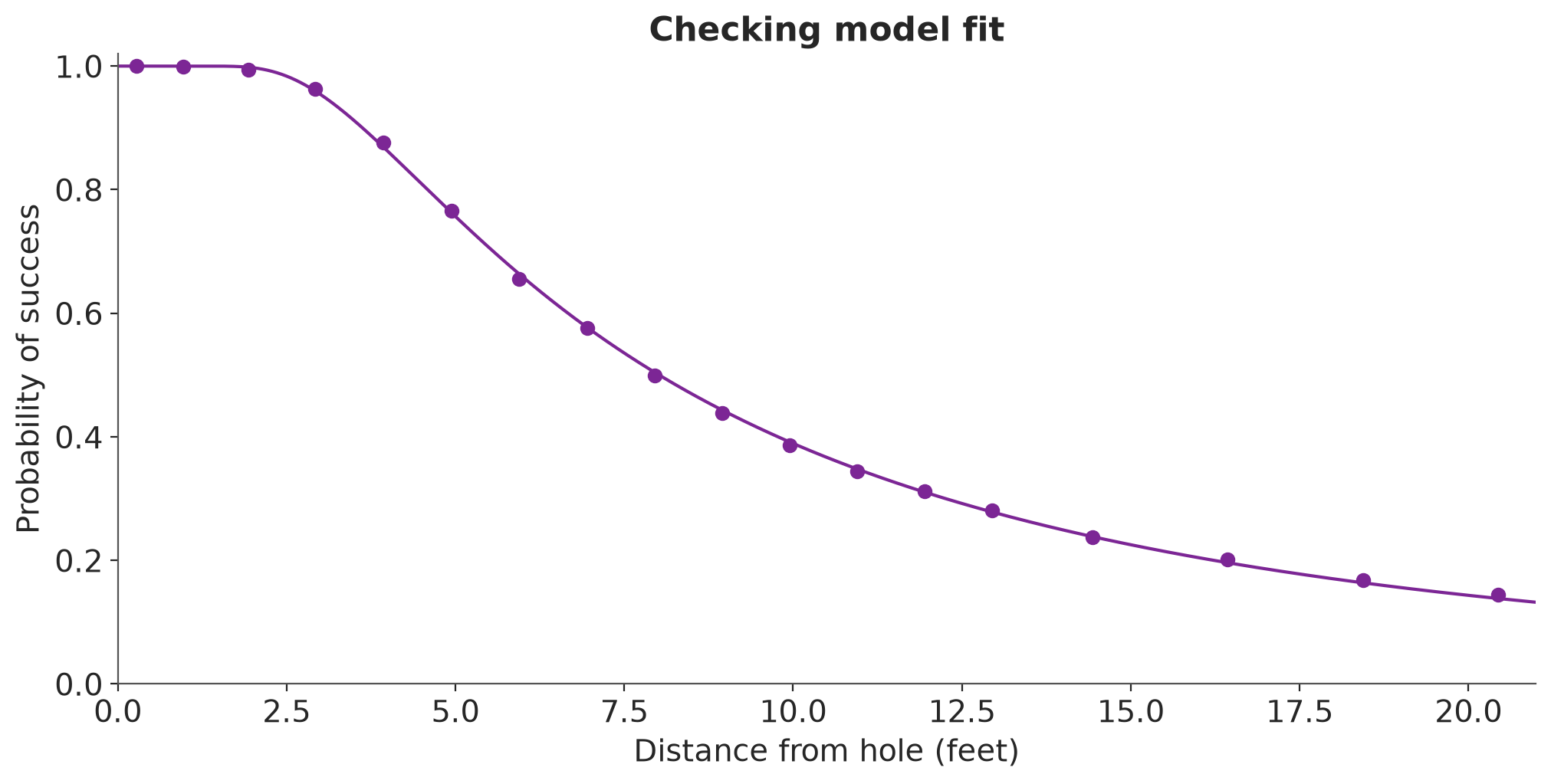
The residuals are now smaller with standard deviation halved, and
there is no obvious pattern. Looking at the posterior of
`distance_tolerance` most of the posterior mass is above 3 and the
posterior is much narrower than the prior and thus likelihood is
informative about it.
```{python}
az.summary(az.from_cmdstanpy(fit_7), var_names=["distance_tolerance"])
```
For the final model we change `overshot` to be a parameter, too. We assume
@Broadie:2018 did use his expertise to choose the value of 1 feet. We use log-normal prior with mean log(1) and standard deviation 0.2 to include that expert information but still have the prior to be relatively weak. We initialize MCMC using the draws from the previous model posterior expect for the new `overshot` parameter and Pathfinder,
```{python}
#| label: golf_angle_distance_binomial_with_proportional_errors_3.stan
#| results: hide
model_8 = CmdStanModel(stan_file=str("golf_angle_distance_binomial_with_proportional_errors_3.stan"))
pth_8 = model_8.pathfinder(
    data=golf_new_data,
    num_paths=40,
    max_lbfgs_iters=100,
)
fit_8 = model_8.sample(
    data=golf_new_data,
    seed=SEED,
    show_progress=False,
    inits=cmdstan_inits(pth_8),
)
```
Here is the result:
```{python}
dt_8 = az.from_cmdstanpy(fit_8)
az.summary(dt_8, var_names="sigma", filter_vars="like")
```
We graph the new data and the fitted model:
```{python}
#| label: fig-golf-fit-8
hats = az.mean(dt_8, round_to="None")
sigma_angle_hat = hats["sigma_angle"].item()
sigma_distance_hat = hats["sigma_distance"].item()
distance_tolerance_8 = hats["distance_tolerance"].item()
overshot_8 = hats["overshot"].item()
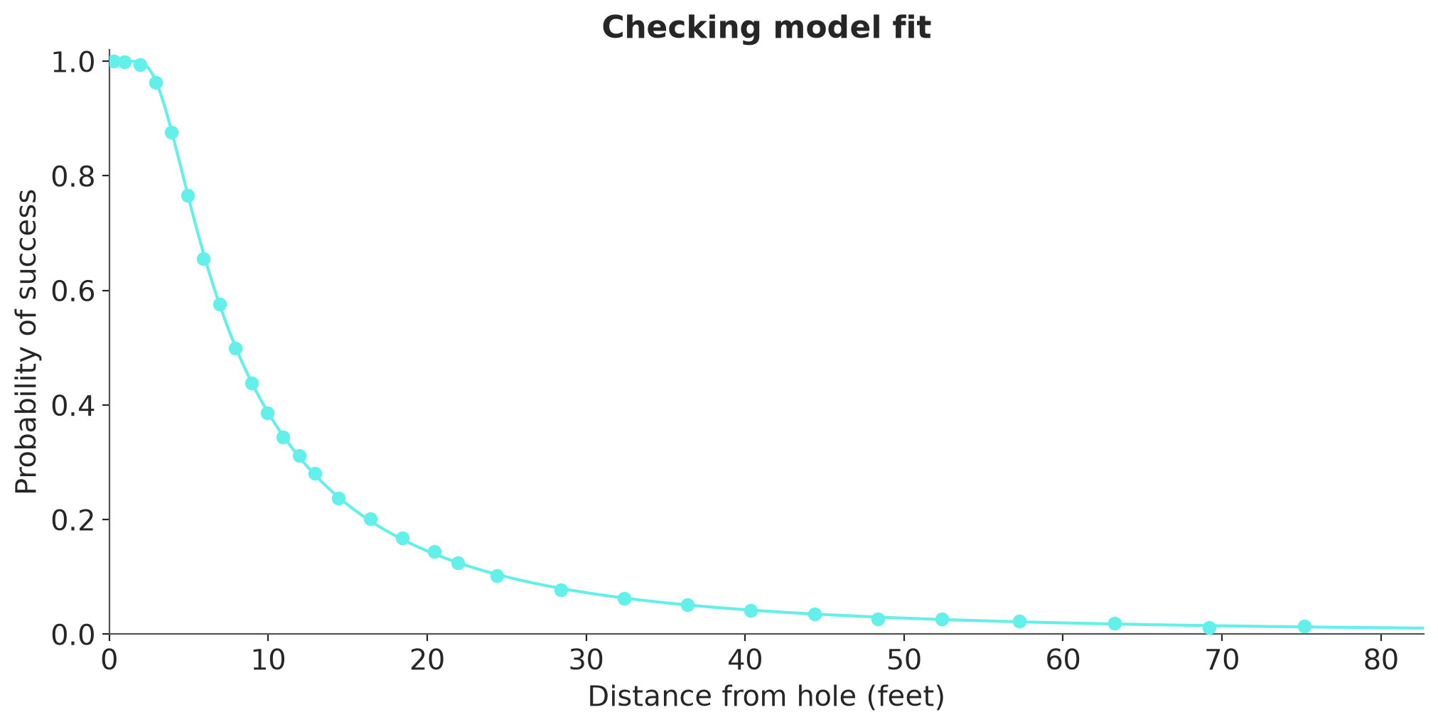
ax = plot_common(title="Checking model fit", plot_observations=False)
ax.set_xlim(0, 1.1 * golf_new["x"].max())
x_grid = np.arange(R - r, 1.1 * golf_new["x"].max(), 0.01)
p_angle_grid = 2 * pz.Normal(0, 1).cdf(np.arcsin((R - r) / x_grid) / sigma_angle_hat) - 1
p_distance_grid = pz.Normal(0, 1).cdf((distance_tolerance_8 - overshot_8) / ((x_grid + overshot_8) * sigma_distance_hat)) - \
    pz.Normal(0, 1).cdf(-overshot_8 / ((x_grid + overshot_8) * sigma_distance_hat))
p_grid = p_angle_grid * p_distance_grid
ax.plot(np.concatenate([[0, R - r], x_grid]),
        np.concatenate([[1, 1], p_grid]), color="C7")
ax.scatter(golf_new["x"], golf_new["y"] / golf_new["n"], color="C7", zorder=3)
```
```{python}
#| label: fig-golf-res-8
posterior_mean_residual_8 = az.mean(dt_8.posterior["residual"], round_to="None")
_, ax = plt.subplots()
ax.set(xlim=(0, 1.1 * golf_new["x"].max()),
       xlabel="Distance from hole (feet)",
       ylabel="y/n - fitted E(y/n)",
       title="Residuals from fitted model"
)
ax.axhline(0, color="gray", linestyle="--")
ax.plot(golf_new["x"], posterior_mean_residual_8)
```
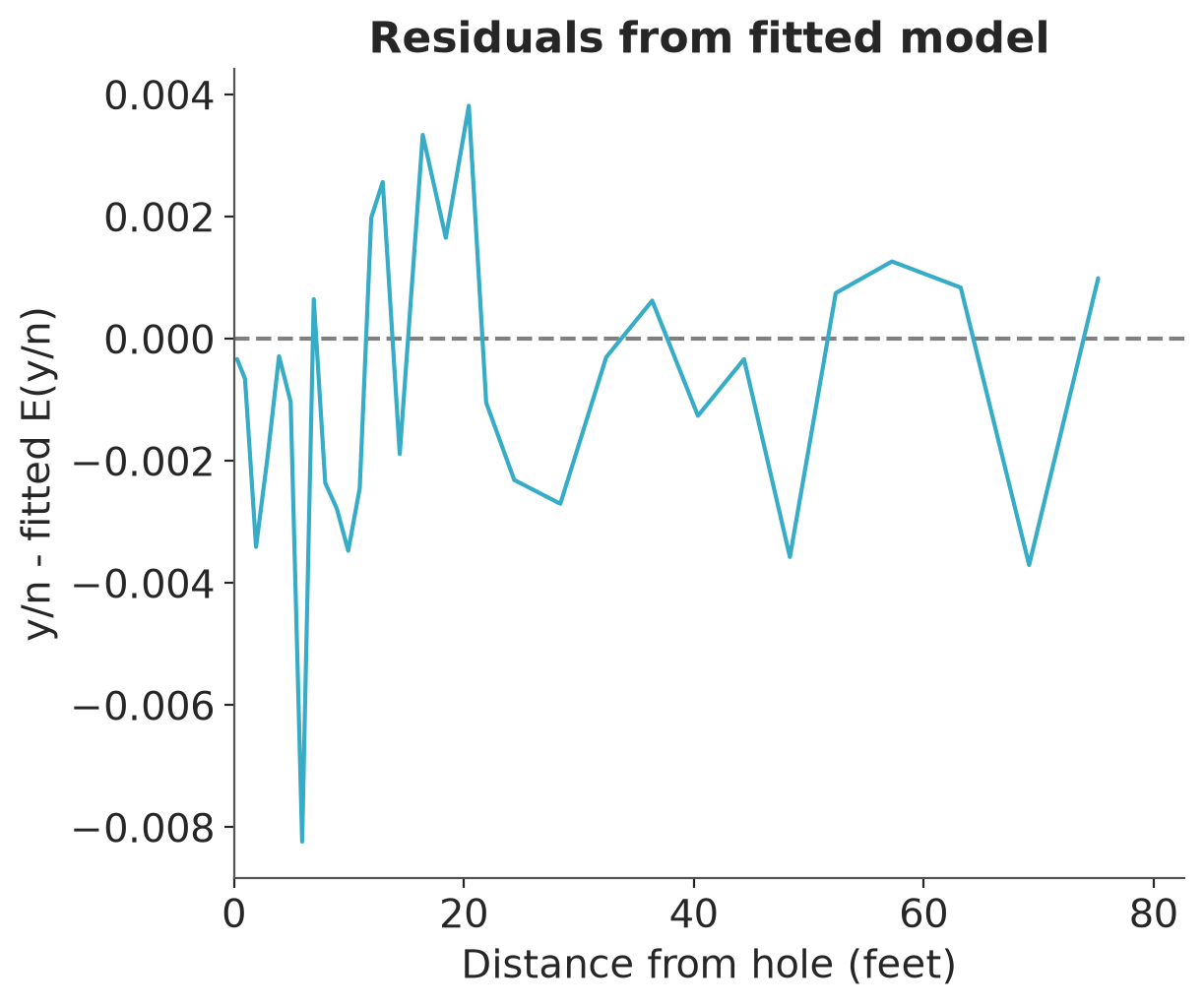
The residuals are very similar to the previous model residuals and with
similar standard deviation. If we examine the posterior marginals
of `distance_tolerance` and `overshot` the standard deviations are
only half from the prior standard deviations, hinting that
likelihood would be weakly informative on these.
```{python}
az.summary(dt_8, var_names=["distance_tolerance", "overshot"])
```
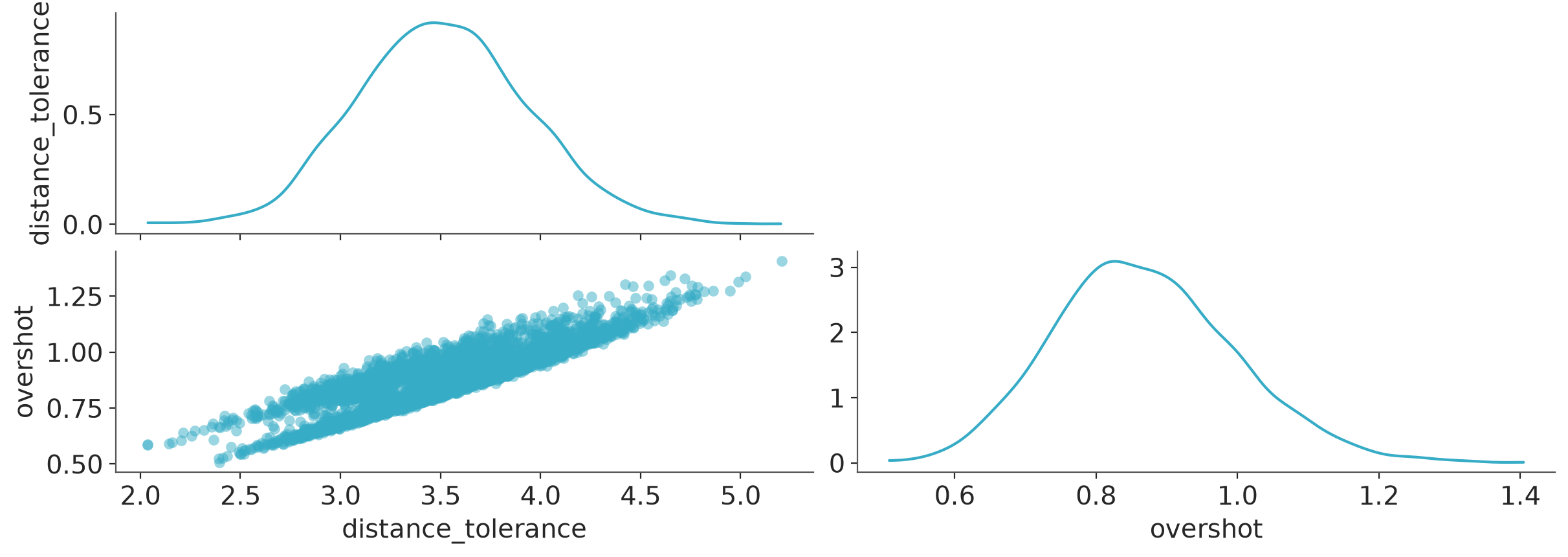
However, when we examine the bivariate posterior we see strong
dependency and their ratio is well informed by the likelihood. The
posterior standard deviation of the ratio is one fifth of the prior
standard deviation. This also explains why adding `overshot` did
not reduce much the residual standard deviation.
```{python}
#| label: fig-mcmc-scatter-tolerance-overshot
az.plot_pair(
    dt_8,
    var_names=["distance_tolerance", "overshot"],
)
```
As we can expect the residual standard deviation to decrease when
we add more parameters, we also use cross-validation to compare the models. As we have one `epsilon` parameter for each observation, we need to use integrated PSIS-LOO. We can compute the integrated `log_lik` with the following stand alone generated quantities code.
```{python}
gq_ll = CmdStanModel(stan_file=str("golf_log_lik.stan"))
gq_ll_7 = CmdStanModel(stan_file=str("golf_log_lik_7.stan"))
gq_ll_8 = CmdStanModel(stan_file=str("golf_log_lik_8.stan"))
```
When calling generated quantities, we pass only the required variables which allowed us to write more compact Stan code for the `log_lik` computation.
```{python}
#| results: hide
def compute_loo(fit, gq_model, data):
    gq = gq_model.generate_quantities(data, previous_fit=fit)
    log_lik = gq.stan_variable("log_lik")
    n_chains = fit.chains
    n_draws = fit.num_draws_sampling
    idata = az.from_dict(
        {"log_likelihood": {"y": log_lik.reshape(n_chains, n_draws, -1)}}
    )
    return az.loo(idata, reff=1)

loo_6 = compute_loo(fit_6, gq_ll, golf_new_data)
loo_7 = compute_loo(fit_7, gq_ll_7, golf_new_data)
loo_8 = compute_loo(fit_8, gq_ll_8, golf_new_data)
```
As we have integrated out the `epsilon` parameters, the effective number of parameters match the number of remaining parameters, except for the last model where `distance_tolerance` and `overshot` parameters are not well informed by the likelihood separately.
```{python}
print(loo_6)
```
```{python}
print(loo_7)
```
```{python}
print(loo_8)
```
Finally we compare the expected predictive performances
```{python}
df_compare = az.compare(
    {
        "Distance tolerance and overshot fixed": loo_6,
        "Distance tolerance parameter and overshot fixed": loo_7,
        "Distance tolerance and overshot parameters": loo_8,
    }
)
df_compare
```
Adding `distance_tolerance` parameter significantly improves the
performance, but adding `overshot` parameter does not improve the
fit. However the model which has both `distance_tolerance` and
`overshot` has posterior that is more informative on what can be
learned about this aspect of the model.
## Binomial with simplified error term
Now we fit a new set of models where the error term epsilon is a
constant rather than a vector. Now epsilon is simply the
probability of completely blowing your shot.
```{python}
#| label: golf_angle_distance_binomial_with_constant_errors.stan
#| results: hide
model_9 = CmdStanModel(stan_file=str("golf_angle_distance_binomial_with_constant_errors.stan"))
fit_9 = model_9.sample(data=golf_new_data, seed=SEED, show_progress=False)
```
Here is the result:
```{python}
dt_9 = az.from_cmdstanpy(fit_9)
az.summary(dt_9, var_names=["sigma_angle", "sigma_distance", "epsilon"])
```
```{python}
#| label: golf_angle_distance_binomial_with_constant_errors_2.stan
#| results: hide
model_10 = CmdStanModel(stan_file=str("golf_angle_distance_binomial_with_constant_errors_2.stan"))
pth_10 = model_10.pathfinder(
    data=golf_new_data,
    num_paths=40,
    max_lbfgs_iters=100,
    inits=cmdstan_inits(fit_9, chains=1)[0],
)
fit_10 = model_10.sample(
    data=golf_new_data,
    seed=SEED,
    show_progress=False,
    inits=cmdstan_inits(pth_10),
)
```
Here is the result:
```{python}
dt_10 = az.from_cmdstanpy(fit_10)
az.summary(dt_10, var_names=["sigma_angle", "sigma_distance", "epsilon"])
```
```{python}
#| label: golf_angle_distance_binomial_with_constant_errors_3.stan
#| results: hide
model_11 = CmdStanModel(stan_file=str("golf_angle_distance_binomial_with_constant_errors_3.stan"))
pth_11 = model_11.pathfinder(
    data=golf_new_data,
    num_paths=40,
    max_lbfgs_iters=100,
    inits=cmdstan_inits(fit_10, chains=1)[0],
)
fit_11 = model_11.sample(
    data=golf_new_data,
    seed=SEED,
    show_progress=False,
    inits=cmdstan_inits(pth_11),
)
```
Here is the result:
```{python}
dt_11 = az.from_cmdstanpy(fit_11)
az.summary(dt_11, var_names=["sigma_angle", "sigma_distance", "distance_tolerance", "overshot", "epsilon"])
```
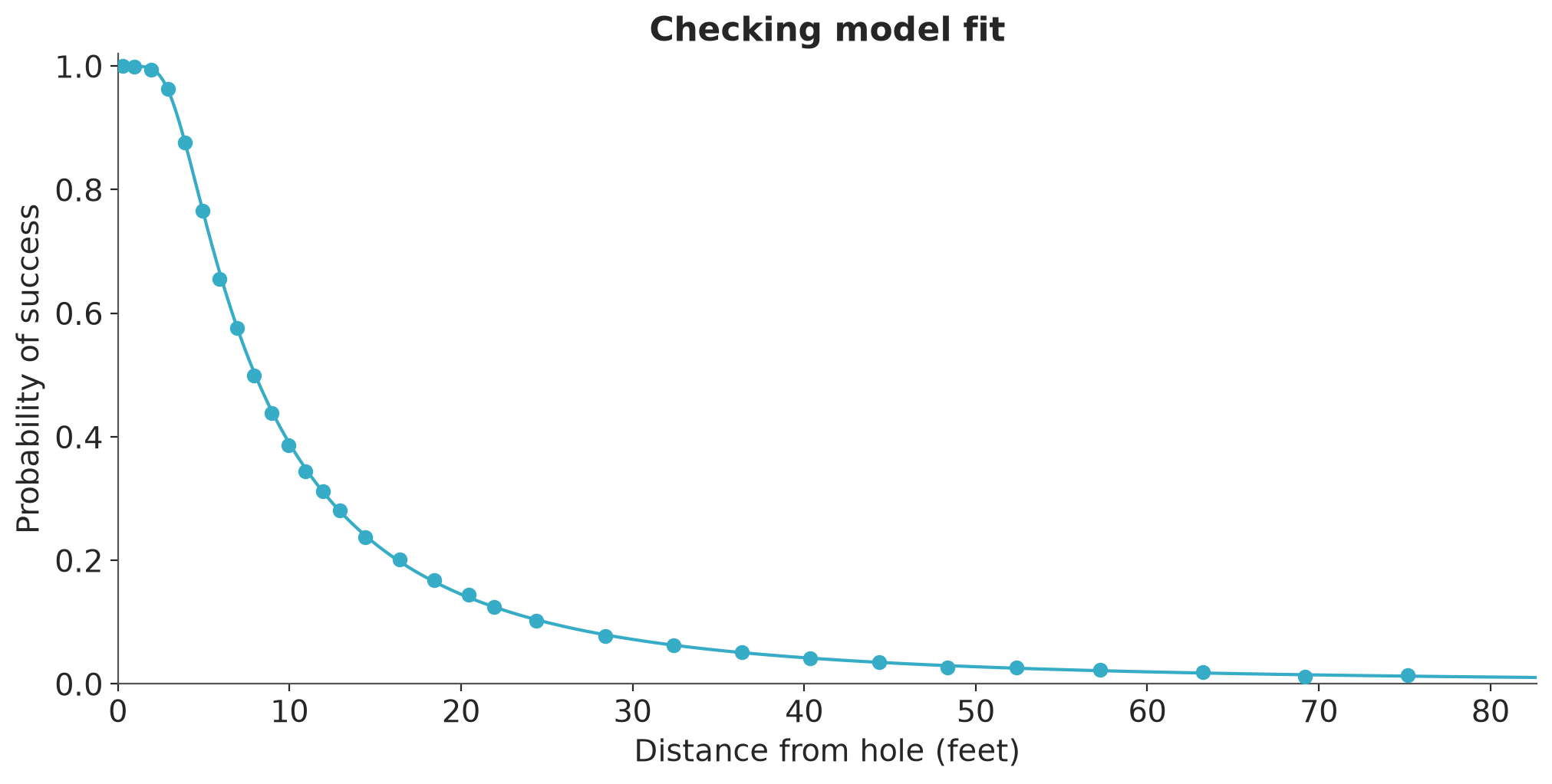
We graph the new data and the fitted model 11:
```{python}
#| label: fig-golf-fit-11
hats = az.mean(dt_11, round_to="None")
sigma_angle_hat = hats["sigma_angle"].item()
sigma_distance_hat = hats["sigma_distance"].item()
distance_tolerance_11 = hats["distance_tolerance"].item()
overshot_11 = hats["overshot"].item()
ax = plot_common(title="Checking model fit", plot_observations=False)
ax.set_xlim(0, 1.1 * golf_new["x"].max())
x_grid = np.arange(R - r, 1.1 * golf_new["x"].max(), 0.01)
p_angle_grid = 2 * pz.Normal(0, 1).cdf(np.arcsin((R - r) / x_grid) / sigma_angle_hat) - 1
p_distance_grid = pz.Normal(0, 1).cdf((distance_tolerance_11 - overshot_11) / ((x_grid + overshot_11) * sigma_distance_hat)) - \
    pz.Normal(0, 1).cdf(-overshot_11 / ((x_grid + overshot_11) * sigma_distance_hat))
p_grid = p_angle_grid * p_distance_grid
ax.plot(np.concatenate([[0, R - r], x_grid]),
        np.concatenate([[1, 1], p_grid]), color="C8")
ax.scatter(golf_new["x"], golf_new["y"] / golf_new["n"], color="C8", zorder=3)
```
```{python}
#| label: fig-golf-res-11
posterior_mean_residual_11 = az.mean(dt_11.posterior["residual"], round_to="None")
_, ax = plt.subplots()
ax.set_xlim(0, 1.1 * golf_new["x"].max())
ax.set_xlabel("Distance from hole (feet)")
ax.set_ylabel("y/n - fitted E(y/n)")
ax.set_title("Residuals from fitted model")
ax.axhline(0, color="gray", linestyle="--")
ax.plot(golf_new["x"], posterior_mean_residual_11)
```
Finally we compare the expected predictive performances
```{python}
#| results: hide
gq_ll_c = CmdStanModel(stan_file=str("golf_log_lik_constant_errors.stan"))
loo_11 = compute_loo(fit_11, gq_ll_c, golf_new_data)
```
We compare the predictive performance of the varying errors and
constant error models.
```{python}
df_compare = az.compare(
    {
        "Model 8 with varying error terms": loo_8,
        "Model 11 with constant error term": loo_11,
    }
)
df_compare
```
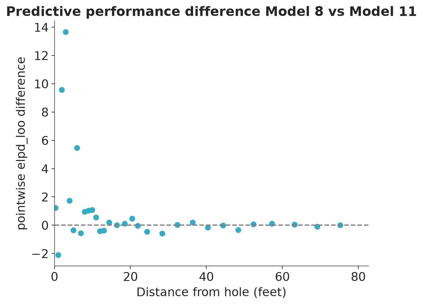
The constant error term is clearly worse with respect to expected
log predictive probability, but that difference is small enough
that it is difficult to see when plotting the prediction on top of
the data.
If we examine the predictive performance difference at different
distances, we see that the constant error model tends to be worse
specifically at short distances.
```{python}
pointwise_elpd_diff = loo_8.elpd_i - loo_11.elpd_i
_, ax = plt.subplots()
ax.scatter(golf_new["x"], pointwise_elpd_diff)
ax.set(xlim=(0, 1.1 * golf_new["x"].max()),
       xlabel="Distance from hole (feet)",
       ylabel="pointwise elpd_loo difference",
       title="Predictive performance difference Model 8 vs Model 11")
ax.axhline(0, color="gray", linestyle="--")
```
<br />
## References {.unnumbered}
<div id="refs"></div>
## Licenses {.unnumbered}
* Code © 2019--2026, Andrew Gelman and Aki Vehtari, licensed under BSD-3.
* Text © 2019--2026, Andrew Gelman and Aki Vehtari, licensed under CC-BY-NC 4.0.