---
title: "Sensitivity and specificity in coronavirus testing"
image: ../social_cards/coronavirus.png
author: "Andrew Gelman and Aki Vehtari"
date: 2022-08-22
date-modified: today
date-format: iso
format:
html:
number-sections: true
code-copy: true
code-download: true
code-tools: true
bibliography: ../casestudies.bib
---
This notebook includes the code for the Bayesian Workflow book
Chapter 19 *Building up to a hierarchical model: Coronavirus
testing*.
## Introduction
In early April, 2020, @Bendavid-Mulaney-Sood-etal:2020a recruited
3330 residents of Santa Clara County, California and tested them
for SARS-CoV-2 antibodies. We re-analyze the data.
```{python}
#| label: setup
#| include: true
#| cache: false
import sys
import warnings

sys.path.insert(0, "..")

import arviz as az
import matplotlib.pyplot as plt
import numpy as np
import pandas as pd

from cmdstanpy import CmdStanModel, disable_logging
from utils import print_stan

disable_logging()
warnings.filterwarnings("ignore")

az.style.use("arviz-variat")
az.rcParams["stats.ci_prob"] = 0.95
plt.rcParams["figure.dpi"] = 100
SEED = 1377
```
## Simple model fit using pooled specificity and sensitivity
```{python}
#| output: asis
sc_model = CmdStanModel(stan_file="santa-clara.stan")
print_stan(sc_model)
```
Compute posterior with data from @Bendavid-Mulaney-Sood-etal:2020a, 11 April 2020
```{python}
#| label: fit_1
fit_1 = sc_model.sample(
    data=dict(
        y_sample=50,
        n_sample=3330,
        y_spec=369 + 30,
        n_spec=371 + 30,
        y_sens=25 + 78,
        n_sens=37 + 85,
    ),
    iter_warmup=int(1e4),
    iter_sampling=int(1e4),
    seed=SEED,
    show_progress=False,
)
idata_1 = az.from_cmdstanpy(fit_1, log_likelihood="log_lik")
idata_1["log_prior"] = idata_1["posterior"]["lprior"].to_dataset()
del idata_1["posterior"]["lprior"]
```
```{python}
az.summary(idata_1)
```
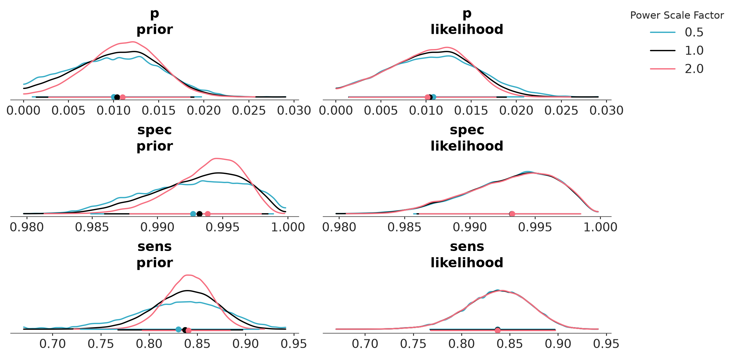
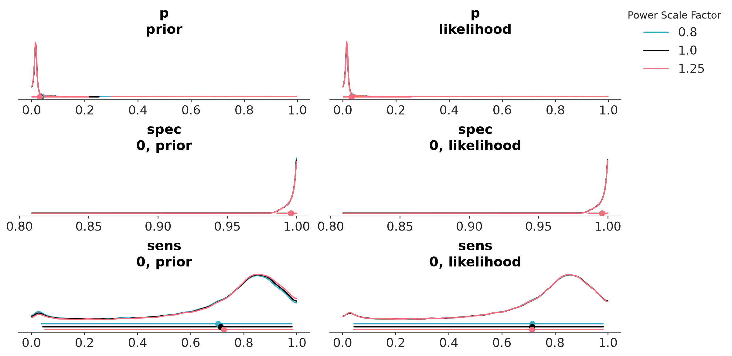
Check prior-likelihood sensitivity using powerscaling
```{python}
az.psense_summary(idata_1)
```
```{python}
#| label: fig-specificity_priorsense_1
az.plot_psense_dist(idata_1,
                    var_names=["~p_sample"],
                    alphas=[0.5, 2],
                    )
```
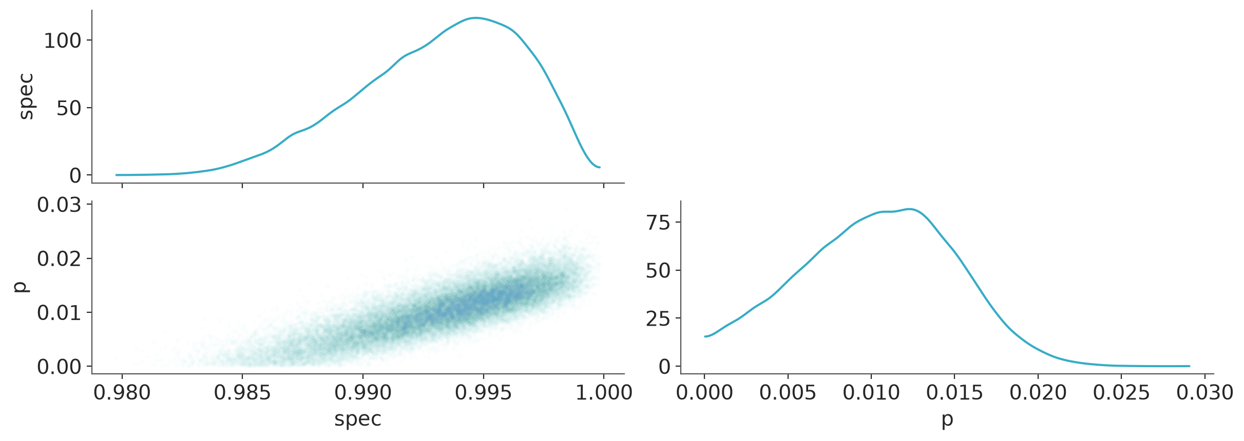
Inference for the population prevalence
```{python}
#| label: fig-scatter
az.plot_pair(idata_1,
             var_names=["spec", "p"],
             visuals={"scatter": {"alpha": 0.01,
                                  "marker":".",}},

             )
```
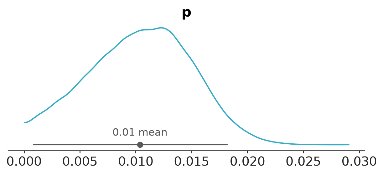
Use the shortest posterior interval, which makes more sense than a central interval because of the skewness of the posterior and the hard boundary at 0.
```{python}
az.plot_dist(idata_1, var_names="p", ci_prob=0.95, ci_kind="hdi");
```
Compute posterior with data from @Bendavid-Mulaney-Sood-etal:2020b, 27 April 2020
```{python}
#| label: fit_2
fit_2 = sc_model.sample(
    data=dict(
        y_sample=50,
        n_sample=3330,
        y_spec=3308,
        n_spec=3324,
        y_sens=130,
        n_sens=157,
    ),
    iter_warmup=int(1e4),
    iter_sampling=int(1e4),
    seed=SEED,
    show_progress=False,
)
idata_2 = az.from_cmdstanpy(fit_2, log_likelihood="log_lik")
idata_2["log_prior"] = idata_2["posterior"]["lprior"].to_dataset()
del idata_2["posterior"]["lprior"]
```
```{python}
az.summary(idata_2, ci_prob=0.95, ci_kind="hdi", kind="stats")
```
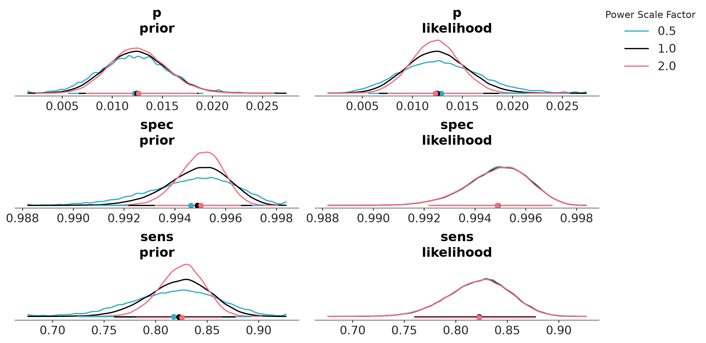
Check prior-likelihood sensitivity using powerscaling
```{python}
az.psense_summary(idata_2, var_names=["~p_sample"])
```
```{python}
#| label: fig-specificity_priorsense_x
az.plot_psense_dist(idata_2, var_names=["~p_sample"], alphas=[0.5, 2])
```
## Hierarchical model for sensitivity and specificity
Hierarchical model that allows sensitivity and specificity to vary across studies.
```{python}
#| output: asis
sc_model_hierarchical = CmdStanModel(stan_file="santa-clara-hierarchical.stan")
print_stan(sc_model_hierarchical)
```
Compute posterior using data from @Bendavid-Mulaney-Sood-etal:2020b 27 April 2020
```{python}
#| label: fit_3a
santaclara_data = dict(
    y_sample=50,
    n_sample=3330,
    J_spec=14,
    y_spec=[0, 368, 30, 70, 1102, 300, 311, 500, 198, 99, 29, 146, 105, 50],
    n_spec=[0, 371, 30, 70, 1102, 300, 311, 500, 200, 99, 31, 150, 108, 52],
    J_sens=4,
    y_sens=[0, 78, 27, 25],
    n_sens=[0, 85, 37, 35],
    logit_spec_prior_scale=1,
    logit_sens_prior_scale=1,
)
fit_3a = sc_model_hierarchical.sample(
    data=santaclara_data,
    iter_warmup=int(1e4),
    iter_sampling=int(1e4),
    adapt_delta=0.99,
    seed=SEED,
    show_progress=False,
)
idata_3a = az.from_cmdstanpy(fit_3a, log_likelihood="log_lik")
idata_3a["log_prior"] = idata_3a["posterior"]["lprior"].to_dataset()
del idata_3a["posterior"]["lprior"]
```
```{python}
var_names = ["p", "spec", "sens",
             "mu_logit_spec", "mu_logit_sens",
             "sigma_logit_spec", "sigma_logit_sens"]

az.summary(idata_3a,
           var_names=var_names,
           coords={"spec_dim_0": [0], "sens_dim_0": [0]},
           ci_prob=0.95,
           ci_kind="hdi",
           kind="stats")
```
```{python}
az.summary(idata_3a,
           var_names=var_names,
           coords={"spec_dim_0": [0], "sens_dim_0": [0]},
           ci_prob=0.95,
           ci_kind="hdi",
           kind="stats")
```
Check prior-likelihood sensitivity using powerscaling
```{python}
az.psense_summary(idata_3a, var_names=["p", "spec", "sens"])
```
```{python}
#| label: fig-specificity_priorsense_2
az.plot_psense_dist(
    idata_3a,
    var_names=["p", "spec", "sens"],
    coords={"spec_dim_0": [0], "sens_dim_0": [0]},
)
```
## Hierarchical model with stronger priors
Compute posterior using data from @Bendavid-Mulaney-Sood-etal:2020b
27 April 2020 and stronger priors
```{python}
santaclara_data["logit_spec_prior_scale"] = 0.3
santaclara_data["logit_sens_prior_scale"] = 0.3
```
MCMC gets sometimes stuck on minor mode, so we initialize with Pathfinder
```{python}
#| label: fit_3b
pth_3b = sc_model_hierarchical.pathfinder(
    data=santaclara_data,
    max_lbfgs_iters=100,
    num_paths=10,
)
fit_3b = sc_model_hierarchical.sample(
    data=santaclara_data,
    iter_warmup=int(1e4),
    iter_sampling=int(1e4),
    adapt_delta=0.99,
    inits=pth_3b.create_inits(),
    seed=SEED,
    show_progress=False,
)
idata_3b = az.from_cmdstanpy(fit_3b, log_likelihood="log_lik")
idata_3b["log_prior"] = idata_3b["posterior"]["lprior"].to_dataset()
del idata_3b["posterior"]["lprior"]
```
```{python}
az.summary(idata_3b,
           var_names=var_names,
           coords={"spec_dim_0": [0], "sens_dim_0": [0]},
           ci_prob=0.95,
           ci_kind="hdi",
           kind="stats")
```
## MRP model
MRP model allowing prevalence to vary by sex, ethnicity, age
category, and zip code. Model is set up to use the ethnicity, age,
and zip categories of @Bendavid-Mulaney-Sood-etal:2020b
```{python}
#| output: asis
sc_model_hierarchical_mrp = CmdStanModel(stan_file="santa-clara-hierarchical-mrp.stan")
print_stan(sc_model_hierarchical_mrp)
```
To fit the model, we need individual-level data.
These data are not publicly available, so just to get the program running,
we take the existing 50 positive tests and assign them at random to the 3330 people.
```{python}
rng = np.random.default_rng(SEED)
N = 3330
y = rng.permutation(np.repeat([0, 1], [3330 - 50, 50]))
```
Here are the counts of each sex, ethnicity, and age from @Bendavid-Mulaney-Sood-etal:2020b.
We don't have zip code distribution but we looked it up and there are 58 zip codes
in Santa Clara County; for simplicity we assume all zip codes are equally likely.
We then assign these traits to people at random.
This is wrong--actually, these variable are correlated in various ways--but, again,
now we have fake data we can use to fit the model.
```{python}
male = rng.permutation(np.repeat([0, 1], [2101, 1229]))
eth = rng.permutation(np.repeat([1, 2, 3, 4], [2118, 623, 266, 306 + 17]))
age = rng.permutation(np.repeat([1, 2, 3, 4], [71, 550, 2542, 167]))
N_zip = 58
zip_codes = rng.integers(1, N_zip + 1, size=3330)
```
Setting up the zip code level predictor.
In this case we will use a random number with mean 50 and standard deviation 20.
These are arbitrary numbers that we chose just to be able to test the centering
and scaling in the model.
In real life we might use %Latino or average income in the zip code
```{python}
x_zip = rng.normal(50, 20, size=N_zip)
```
Setting up the poststratification table.
For simplicity we assume there are 1000 people in each cell in the county.
Actually we'd want data from the Census.
```{python}
J = 2 * 4 * 4 * N_zip
N_pop = np.full(J, 1000)
```
Put together the data and fit the model
```{python}
#| label: fit_4
santaclara_mrp_data = dict(
    N=N,
    y=y.tolist(),
    male=male.tolist(),
    eth=eth.tolist(),
    age=age.tolist(),
    zip=zip_codes.tolist(),
    N_zip=N_zip,
    x_zip=x_zip.tolist(),
    J_spec=14,
    y_spec=[0, 368, 30, 70, 1102, 300, 311, 500, 198, 99, 29, 146, 105, 50],
    n_spec=[0, 371, 30, 70, 1102, 300, 311, 500, 200, 99, 31, 150, 108, 52],
    J_sens=4,
    y_sens=[0, 78, 27, 25],
    n_sens=[0, 85, 37, 35],
    logit_spec_prior_scale=0.3,
    logit_sens_prior_scale=0.3,
    coef_prior_scale=0.5,
    J=J,
    N_pop=N_pop.tolist(),
)
fit_4 = sc_model_hierarchical_mrp.sample(
    data=santaclara_mrp_data,
    seed=SEED,
    show_progress=False,
)
idata_4 = az.from_cmdstanpy(fit_4)
```
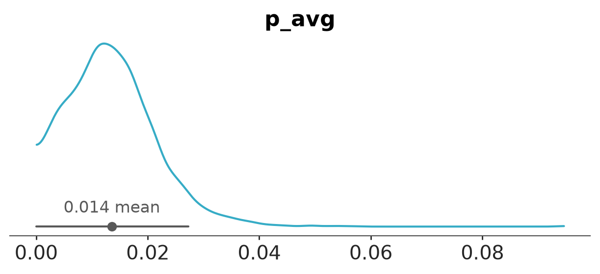
Show inferences for some model parameters. In addition to `p_avg`, the population
prevalence, we also look at the inferences for the first three
poststratification cells just to check that everything makes sense
```{python}
print_variables_mrp = [
    "p_avg", "b", "a_age", "a_eth",
    "sigma_eth", "sigma_age", "sigma_zip",
    "mu_logit_spec", "sigma_logit_spec",
    "mu_logit_sens", "sigma_logit_sens",
    "p_pop",
]
az.summary(idata_4, var_names=print_variables_mrp,
coords={"p_pop_dim_0": [0, 1, 2]}, kind="stats")
```
```{python}
az.plot_dist(idata_4, var_names="p_avg", ci_prob=0.95, ci_kind="hdi");
```
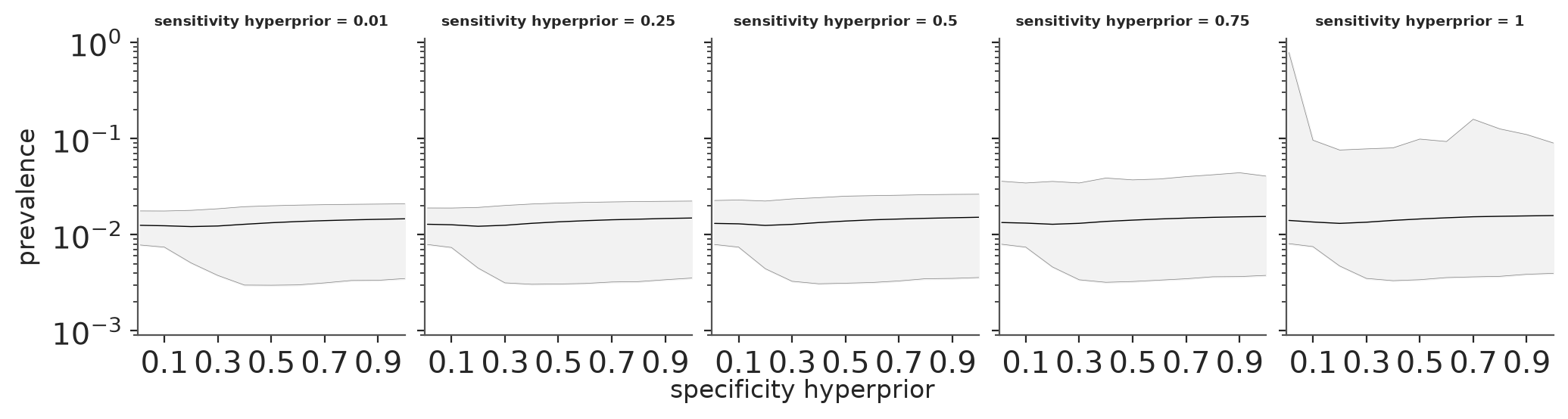
## Additional prior sensitivity analysis
```{python}
pos_tests = [78, 27, 25]
tests = [85, 37, 35]
sens_df = pd.DataFrame(
    {"pos_tests": pos_tests, "tests": tests,
     "sample_sens": [p / t for p, t in zip(pos_tests, tests)]}
)

neg_tests = [368, 30, 70, 1102, 300, 311, 500, 198, 99, 29, 146, 105, 50]
tests = [371, 30, 70, 1102, 300, 311, 500, 200, 99, 31, 150, 108, 52]
spec_df = pd.DataFrame(
    {"neg_tests": neg_tests, "tests": tests,
     "sample_spec": [n / t for n, t in zip(neg_tests, tests)]}
)

pos_tests = [50]
tests = [3330]
unk_df = pd.DataFrame(
    {"pos_tests": pos_tests, "tests": tests,
     "sample_prev": [p / t for p, t in zip(pos_tests, tests)]}
)
```
Stan model for prior sensitivity analysis
```{python}
#| output: asis
sens_model = CmdStanModel(stan_file="prior-sensitivity.stan")
print_stan(sens_model)
```
Data
```{python}
data = dict(
    K_pos=len(sens_df),
    N_pos=sens_df["tests"].tolist(),
    n_pos=sens_df["pos_tests"].tolist(),
    K_neg=len(spec_df),
    N_neg=spec_df["tests"].tolist(),
    n_neg=spec_df["neg_tests"].tolist(),
    K_unk=len(unk_df),
    N_unk=unk_df["tests"].tolist(),
    n_unk=unk_df["pos_tests"].tolist(),
)
```
Empty data frame to store posterior intervals with different priors
```{python}
ribbon_df = pd.DataFrame(
    columns=["sigma_sens", "sigma_spec", "prev05", "prev50", "prev95"]
)
```
Loop over different prior parameter values
```{python}
#| label: loop-over-prior-values
#| cache: true
sigma_senss = [0.01, 0.25, 0.5, 0.75, 1]
sigma_specss = [0.01, 0.1, 0.2, 0.3, 0.4, 0.5, 0.6, 0.7, 0.8, 0.9, 1.0]
for sigma_sens in sigma_senss:
    for sigma_spec in sigma_specss:
        data2 = {**data,
                 "sigma_sigma_logit_sens": sigma_sens,
                 "sigma_sigma_logit_spec": sigma_spec}
        fit = sens_model.sample(
            data=data2,
            iter_warmup=int(5e4),
            iter_sampling=int(5e4),
            seed=1234,
            adapt_delta=0.95,
            show_progress=False,
        )
        pis = fit.stan_variable("pi")
        ribbon_df = pd.concat(
            [ribbon_df,
             pd.DataFrame({
                 "sigma_sens": [f"sensitivity hyperprior = {sigma_sens}"],
                 "sigma_spec": [sigma_spec],
                 "prev05": [np.quantile(pis, 0.05)],
                 "prev50": [np.quantile(pis, 0.5)],
                 "prev95": [np.quantile(pis, 0.95)],
             })],
            ignore_index=True,
        )
```
```{python}
#| label: fig-prior-sensitivity-2
sens_levels = [f"sensitivity hyperprior = {s}" for s in sigma_senss]
fig, axes = plt.subplots(1, len(sens_levels), figsize=(10, 2.5),
                         sharey=True, sharex=True)
for ax, level in zip(axes, sens_levels):
    sub = ribbon_df[ribbon_df["sigma_sens"] == level].sort_values("sigma_spec")
    x = sub["sigma_spec"].to_numpy(dtype=float)
    y05 = sub["prev05"].to_numpy(dtype=float)
    y50 = sub["prev50"].to_numpy(dtype=float)
    y95 = sub["prev95"].to_numpy(dtype=float)
    ax.fill_between(x, y05, y95, color="0.95")
    ax.plot(x, y50, color="black", linewidth=0.5)
    ax.plot(x, y05, color="0.5", linewidth=0.25)
    ax.plot(x, y95, color="0.5", linewidth=0.25)
    ax.set(yscale="log",
           ylim=(0.0009, 1.1),
           yticks=[0.001, 0.01, 0.1, 1],
           xlim=(0, 1),
           xticks=[0.1, 0.3, 0.5, 0.7, 0.9])
    ax.set_title(level, fontsize=7)
fig.text(0.5, -0.03, "specificity hyperprior", ha="center")
fig.text(-0.02, 0.5, "prevalence", va="center", rotation=90);
```
## References {.unnumbered}
<div id="refs"></div>
## Licenses {.unnumbered}
* Code © 2022--2025, Andrew Gelman and Aki Vehtari, licensed under BSD-3.
* Text © 2022--2025, Andrew Gelman and Aki Vehtari, licensed under CC-BY-NC 4.0.