---
title: "Illustration of simple problematic posteriors"
image: ../social_cards/problems.png
author: "Aki Vehtari"
date: 2021-06-10
date-modified: today
date-format: iso
format:
html:
number-sections: true
code-copy: true
code-download: true
code-tools: true
bibliography: ../casestudies.bib
---
This notebook includes the code for Bayesian Workflow book Section
12.3 *Failure modes and steps forward*.
## Introduction
This case study demonstrates using simple examples the most common
failure modes in Markov chain Monte Carlo based Bayesian inference,
how to recognize these using the diagnostics, and how to fix the
problems.
**Load packages**
```{python}
import sys
import warnings

sys.path.insert(0, "..")

import numpy as np
import pandas as pd
import matplotlib.pyplot as plt
from pathlib import Path
from cmdstanpy import CmdStanModel, disable_logging
import arviz as az

from utils import print_stan

# Set plotting style
az.style.use("arviz-variat")
plt.rcParams["figure.dpi"] = 100

warnings.filterwarnings("ignore")
disable_logging()

SEED = 48927
np.random.seed(SEED)
```
## Improper posterior
An unbounded likelihood without a proper prior can lead to an
improper posterior. We recommend to always use proper priors
(integral over a proper distribution is finite) to guarantee proper
posteriors.
A commonly used model that can have unbounded likelihood is
logistic regression with complete separation in data.
### Data
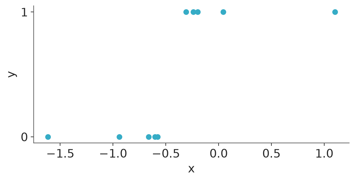
Univariate continous predictor $x$, binary target $y$, and the two classes are completely separable, which leads to unbounded likelihood.
```{python}
rng = np.random.default_rng(SEED + 4)
M = 1
N = 10
# x = np.sort(rng.normal(size=(N, M)), axis=0)
x = np.array(
    [
        [-1.61675183],
        [-0.94052670],
        [-0.66244057],
        [-0.60232373],
        [-0.57819996],
        [-0.30952063],
        [-0.23880912],
        [-0.19792298],
        [0.04290007],
        [1.10171923],
    ]
)
y = np.repeat([0, 1], N / 2)
data_logit = {"M": M, "N": N, "x": x, "y": y}
```
```{python}
#| label: fig-separable_data
df = pd.DataFrame({"x": x.flatten(), "y": y})
_, ax = plt.subplots(figsize=(6, 3))

ax.scatter(df["x"], df["y"])
ax.set(yticks=[0, 1], xlabel="x", ylabel="y");
```
### Model
We use the following Stan logistic regression model, where we have "forgot" to include prior for the coefficient `beta`.
```{python}
mod_logit = CmdStanModel(stan_file=str("logit_glm.stan"))
print_stan(mod_logit)
```
Sample
```{python}
#| label: fit_logit
fit_logit = mod_logit.sample(data=data_logit, seed=SEED, show_progress=False)
dt_logit = az.from_cmdstanpy(fit_logit)
```
### Convergence diagnostics
When running Stan, we get warnings. We can also
explicitly check the inference diagnostics:
```{python}
az.diagnose(dt_logit)
```
We can also check $\widehat{R}$ and effective sample size (ESS) diagnostics[@Vehtari-Gelman-Simpson-etal:2021]
```{python}
az.summary(dt_logit)
```
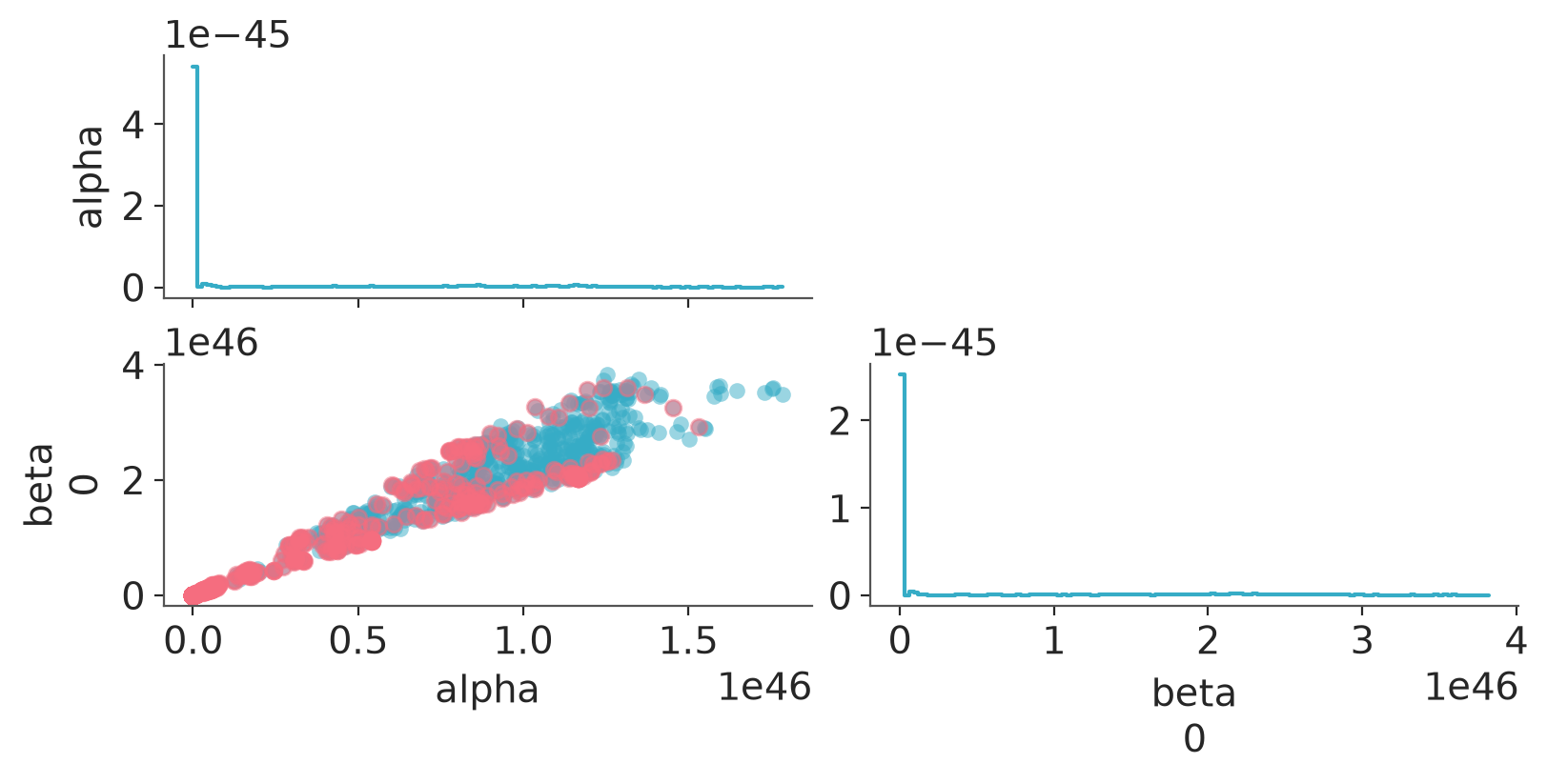
We see that $\widehat{R}$ for both `alpha` and `beta` are about 3 or 4 and ESS is about 4, which indicate that the chains are not mixing at all.
The above diagnostics refer to a documentation ([https://mc-stan.org/misc/warnings](https://mc-stan.org/misc/warnings)) that mentions possibility to adjust the sampling algorithm options (e.g., increasing `adapt_delta` and `max_treedepth`), but it is better first to investigate the posterior.
The following Figure shows the posterior draws as marginal histograms and joint scatterplots. The range of the values is huge, which is typical for improper posterior, but the values of `alpha` and `beta` in any practical application are likely to have much smaller magnitude. In this case, increasing `adapt_delta` and `max_treedepth` would not have solved the problem, and would have just caused waste of modeler and computation time.
```{python}
#| label: fig-separable_pairs
az.plot_pair(
    dt_logit,
    marginal_kind="hist",
    figure_kwargs={"figsize": (8, 4)},
    visuals={"divergence": True},
)
```
#### Stan compiler pedantic check
The above diagnostics are applicable with any probabilistic programming framework. Stan compiler can also recognize some common problems. By default the pedantic mode is not enabled, but we can use option `pedantic = TRUE` at compilation time.
The pedantic check correctly warns that `alpha` and `beta` don't have priors.
### A fixed model with proper priors
We add proper weak priors and rerun inference.
```{python}
mod_logit2 = CmdStanModel(stan_file="logit_glm2.stan")
print_stan(mod_logit2)
```
Sample
```{python}
#| label: fit_logit2
fit_logit2 = mod_logit2.sample(data=data_logit, seed=SEED, show_progress=False)
dt_logit2 = az.from_cmdstanpy(fit_logit2)
```
#### Convergence diagnostics
There were no convergence warnings. We can also
explicitly check the inference diagnostics:
```{python}
az.diagnose(dt_logit2)
```
We check $\widehat{R}$ and ESS values, which in this case all look good.
```{python}
az.summary(dt_logit2)
```
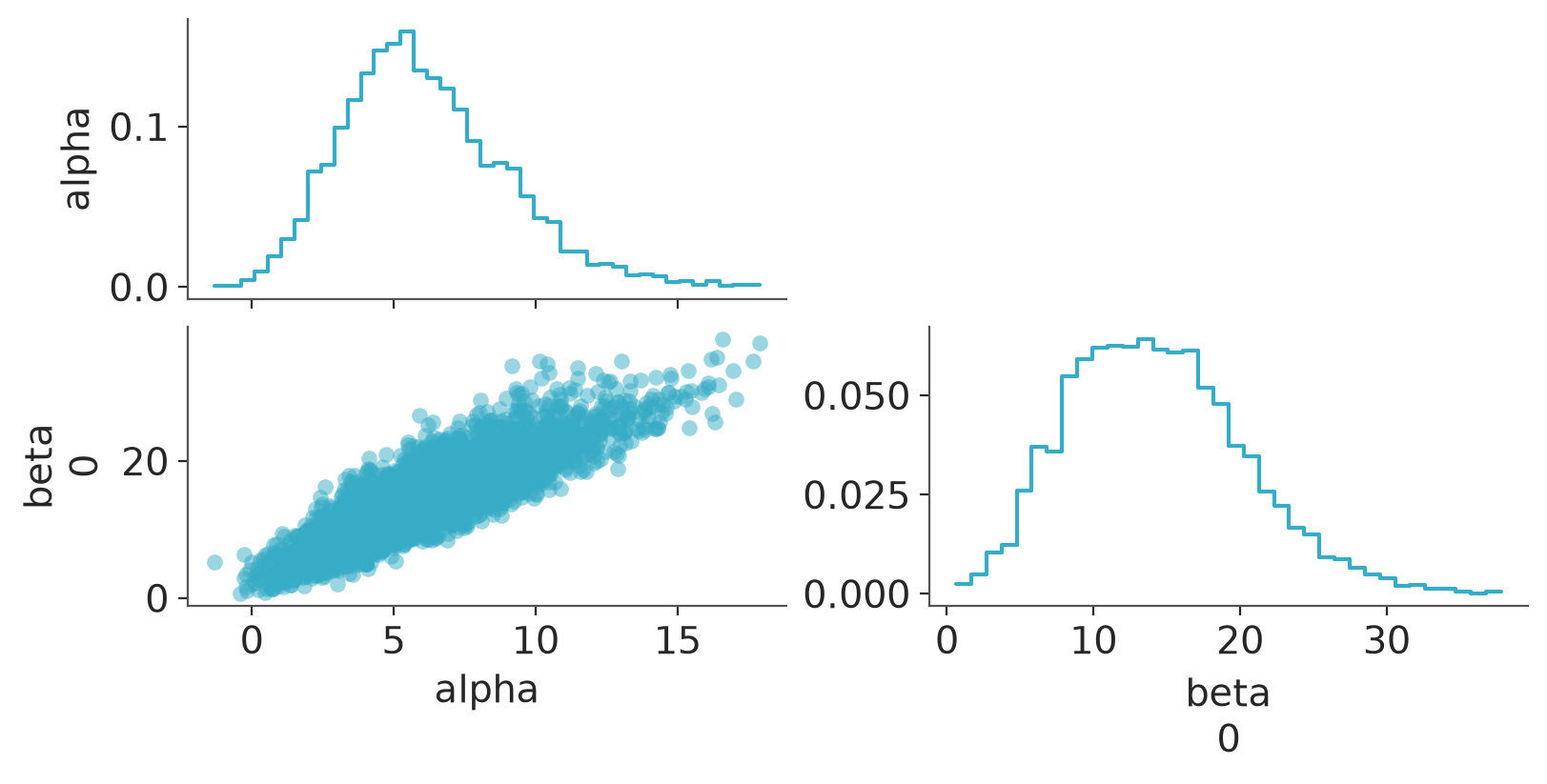
The following figure shows the more reasonable marginal histograms
and joint scatterplots of the posterior sample.
```{python}
#| label: fig-separable_prior_pairs
az.plot_pair(
    dt_logit2,
    marginal_kind="hist",
    figure_kwargs={"figsize": (8, 4)},
    visuals={"divergence": True},
)
```
## A model with unused parameter
When writing and editing models, a common mistake is to declare a parameter, but not use it in the model. If the parameter is not used at all, it doesn't have proper prior and the likelihood doesn't provide information about that parameter, and thus the posterior along that parameter is improper. We use the previous logistic regression model with proper priors on `alpha` and `beta`, but include extra parameter declaration `real gamma`.
### Model
```{python}
mod_logit3 = CmdStanModel(stan_file="logit_glm3.stan")
print_stan(mod_logit3)
```
Sample
```{python}
#| label: fit_logit3
fit_logit3 = mod_logit3.sample(data=data_logit, seed=SEED, show_progress=False)
dt_logit3 = az.from_cmdstanpy(fit_logit3)
```
#### Convergence diagnostics
There is sampler warning. We can also explicitly call inference
diagnostics:
```{python}
az.diagnose(dt_logit3)
```
Instead of increasing `max_treedepth`, we check the other convergence diagnostics.
```{python}
az.summary(dt_logit3)
```
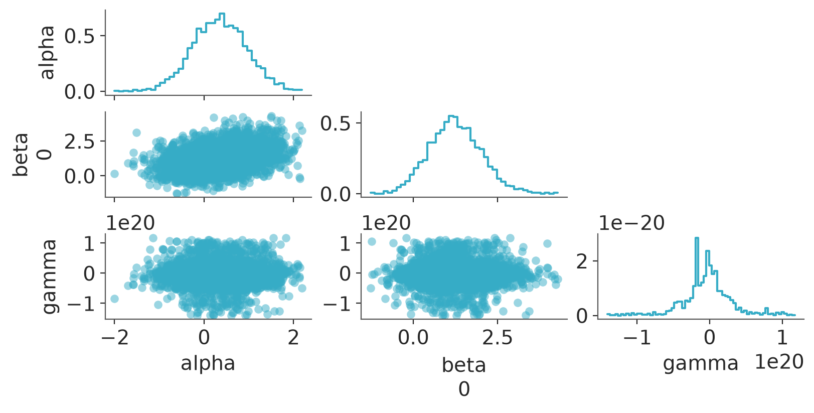
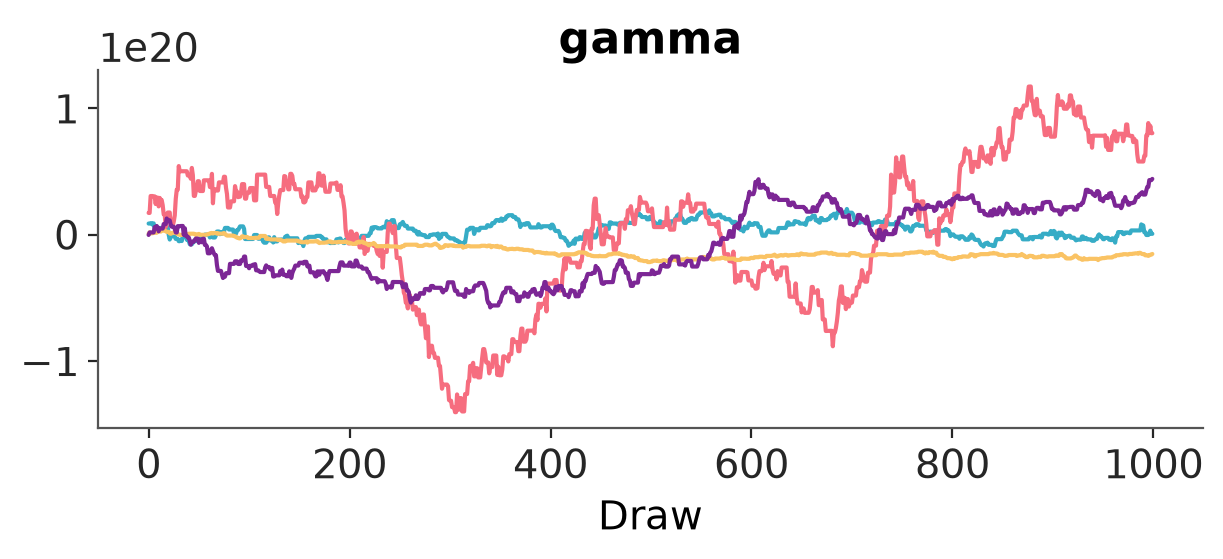
$\widehat{R}$, ESS look good for `alpha` and `beta`, but really bad for `gamma`, clearly pointing where to look for problems in the model code. The histogram of `gamma` posterior draws show huge magnitude of values (values larger than $10^{20}$) indicating improper posterior.
```{python}
#| label: fig-unusedparam_pairs
az.plot_pair(
    dt_logit3,
    marginal_kind="hist",
    figure_kwargs={"figsize": (8, 4)},
    visuals={"divergence": True},
)
```
Non-mixing is well diagnosed by $\widehat{R}$ and ESS, but the following Figure shows one of the rare cases where trace plots are useful to illustrate the type of non-mixing in case of improper uniform posterior for one the parameters.
```{python}
#| label: fig-unusedparam_trace
az.plot_trace(dt_logit3, var_names=["gamma"])
```
### Stan compiler pedantic check
Stan compiler pedantic check also recognizes that parameter `gamma` was declared but was not used in the density calculation.
## A posterior with two parameters competing
Sometimes the models have two or more parameters that have similar or exactly the same role. We illustrate this by adding an extra column to the previous data matrix. Sometimes the data matrix is augmented with a column of 1's to present the intercept effect. In this case that is redundant as our model has the explicit intercept term `alpha`, and this redundancy will lead to problems.
### Data
```{python}
M = 2
N = 1000
x = np.column_stack([np.ones(N), np.sort(np.random.randn(N))])
y = ((x[:, 0] + np.random.randn(N) / 2) > 0).astype(int)
data_logit4 = {"M": M, "N": N, "x": x, "y": y}
```
### Model
We use the previous logistic regression model with proper priors (and no extra `gamma`).
```{python}
print_stan(mod_logit2)
```
Sample
```{python}
#| label: fit_logit4
mod_logit4 = CmdStanModel(stan_file="logit_glm2.stan")
fit_logit4 = mod_logit4.sample(data=data_logit4, seed=SEED, show_progress=False)
dt_logit4 = az.from_cmdstanpy(fit_logit4)
```
The Stan sampling time per chain with the original data matrix was less than 0.1s per chain. Now the Stan sampling time per chain is several seconds, which is suspicious. There are no automatic convergence diagnostic warnings and checking other diagnostics don't show anything really bad.
### Convergence diagnostics
```{python}
az.diagnose(dt_logit4)
```
```{python}
az.summary(dt_logit4)
```
ESS estimates are above the recommended diagnostic thresholds [@Vehtari-Gelman-Simpson-etal:2021], but lower than what we would expect in general from Stan for such a lower dimensional problem.
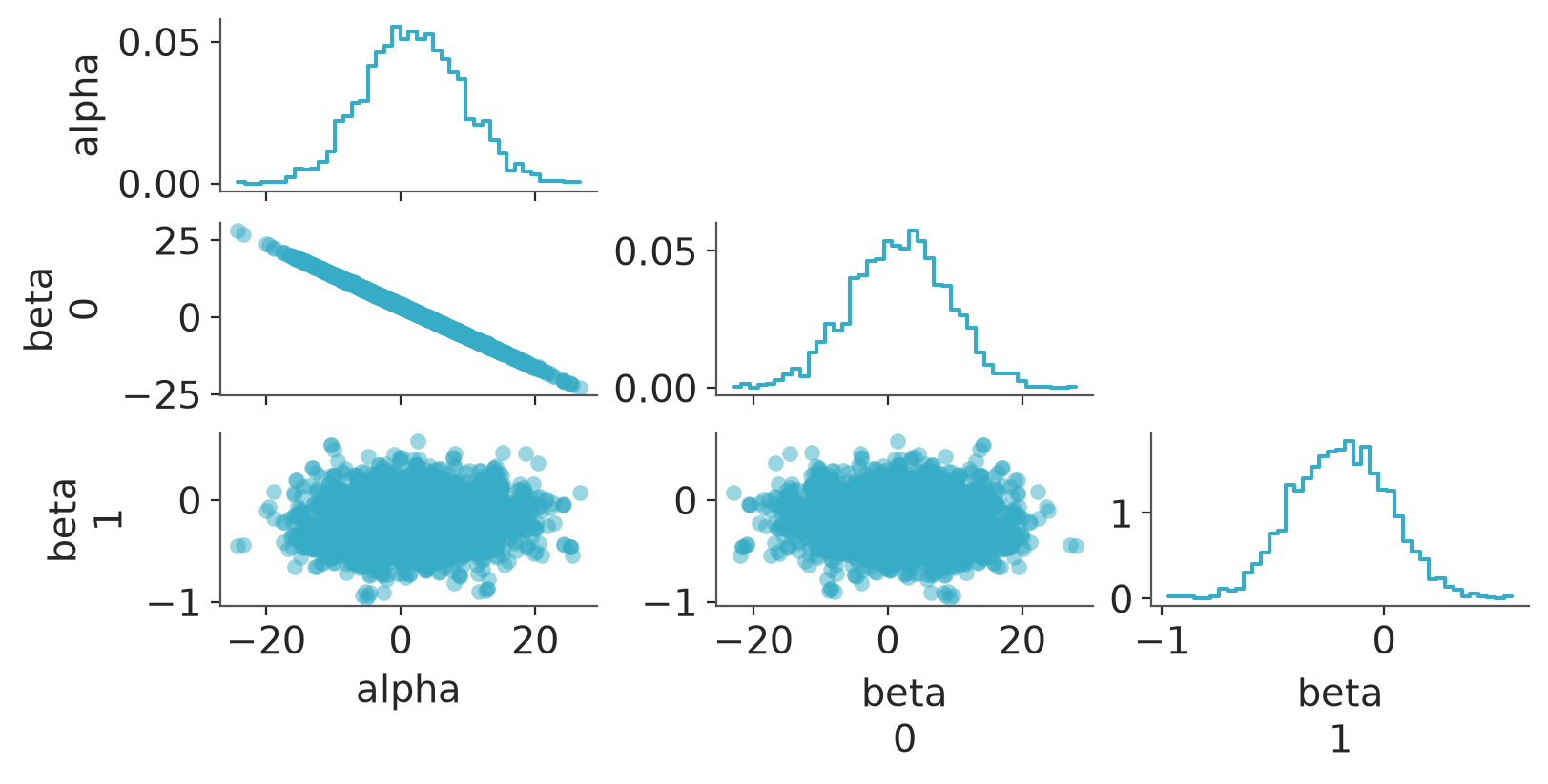
The following figure shows marginal histograms and joint
scatterplots, and we can see that `alpha` and `beta_0` are highly
correlated.
```{python}
#| label: fig-competing_params_pairs
az.plot_pair(
    dt_logit4,
    marginal_kind="hist",
    figure_kwargs={"figsize": (8, 4)},
    visuals={"divergence": True},
)
```
We can compute the correlation.
```{python}
posterior_samples = az.extract(dt_logit4)
alpha_samples = posterior_samples["alpha"].values
beta_samples = posterior_samples["beta"].values
correlation = np.corrcoef(alpha_samples, beta_samples)[0, 1]
print(f"Correlation: {correlation:.2f}")
```
The numerical value for the correlation is $-1$. The
correlation close to 1 can happen also from other reasons (see the next example), but one possibility is that parameters have similar role in the model. Here the reason is the constant column in $x$, which we put there for the demonstration purposes. We may have constant column, for example, if the predictor matrix is augmented with the intercept predictor, or if the observed data or subdata used in the specific analysis happens to have only one unique value.
### Stan compiler pedantic check
Stan compiler pedantic check examining the code can't
recognize this issue, as the problem depends also on the data.
## A posterior with very high correlation
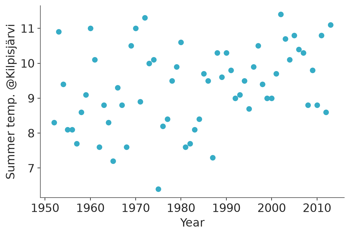
In the previous example the two parameters had the same role in the model, leading to high posterior correlation. High posterior correlations are common also in linear models when the predictor values are far from 0. We illustrate this with a linear regression model for the summer temperature in Kilpisjärvi, Finland, 1952--2013. We use the year as the covariate $x$ without centering it.
### Data
The data are Kilpisjärvi summer month temperatures 1952-2013
measured by Finnish Meteorological Institute.
```{python}
data_kilpis = pd.read_csv("data/kilpisjarvi-summer-temp.csv", sep=";")
M = 1
N = len(data_kilpis)
x = data_kilpis["year"].values.reshape(-1, 1)
y = data_kilpis.iloc[:, 4].values
data_lin = {"M": M, "N": N, "x": x, "y": y}
```
```{python}
#| label: fig-kilpisjarvi_data
_, ax = plt.subplots(figsize=(6, 4))
ax.scatter(x, y)
ax.set(xlabel="Year", ylabel="Summer temp. @Kilpisjärvi")
```
### Model
We use the following Stan linear regression model
```{python}
mod_lin = CmdStanModel(stan_file="linear_glm_kilpis.stan")
print_stan(mod_lin)
```
```{python}
#| label: fit_lin_kilpis
fit_lin = mod_lin.sample(data=data_lin, seed=SEED, show_progress=False)
dt_lin = az.from_cmdstanpy(fit_lin)
```
#### Convergence diagnostics
Stan gives a warning: There were X transitions after warmup that exceeded the maximum treedepth. As in the previous example, there are no other warnings.
```{python}
az.diagnose(dt_lin)
```
```{python}
az.summary(dt_lin)
```
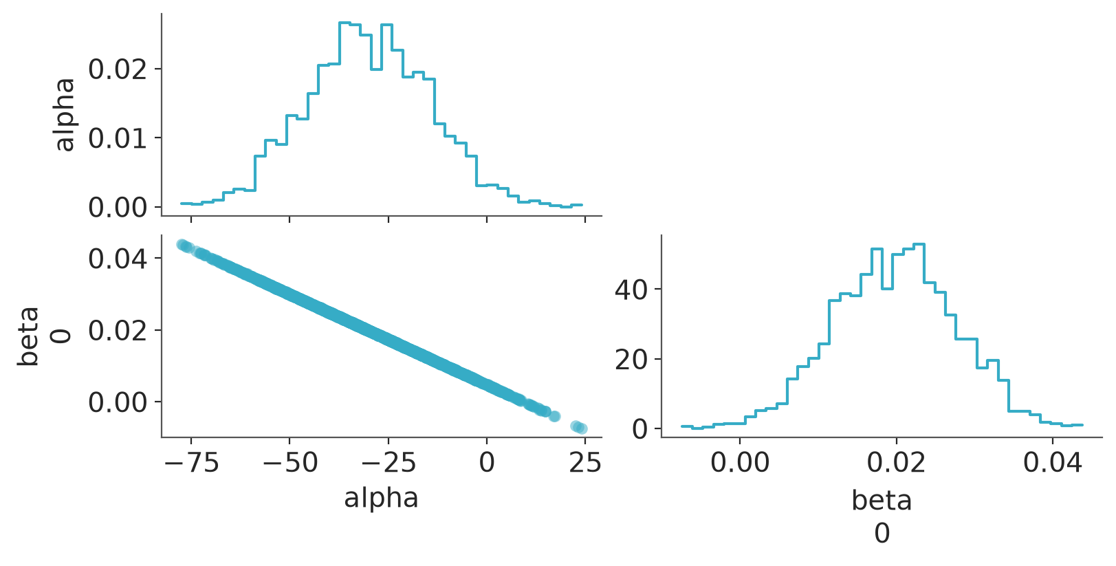
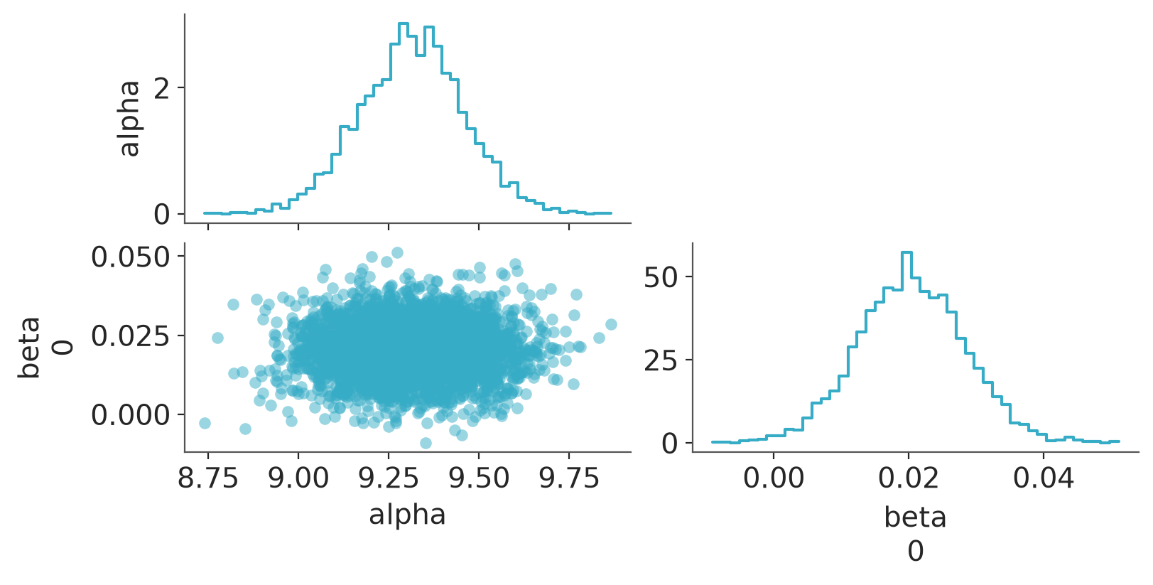
ESS estimates are above the diagnostic threshold, but lower than we would expect for such a low dimensional model, unless there are strong posterior correlations. The following figure shows the marginal histograms and joint scatterplot for `alpha` and `beta_0`, which shows they are very highly correlated.
```{python}
#| label: fig-correlating_params_pairs
az.plot_pair(
    dt_lin,
    var_names=["alpha", "beta"],
    marginal_kind="hist",
    figure_kwargs={"figsize": (8, 4)},
    visuals={"divergence": True},
)
```
Here the reason is that the $x$ values are in the range 1952--2013, and the intercept `alpha` denotes the temperature at year 0, which is very far away from the range of observed $x$. If the intercept `alpha` changes, the slope `beta` needs to change too. The high correlation makes the inference slower, and we can make it faster by centering $x$. Here we simply subtract 1982.5 from the predictor `year`, so that the mean of $x$ is 0. We could also include the centering and back transformation in the Stan code.
### Centered data
```{python}
x_centered = data_kilpis["year"].values - 1982.5
data_lin = {"M": M, "N": N, "x": np.atleast_2d(x_centered).T, "y": y}
```
```{python}
#| label: fit_lin_kilpis_centered_data
fit_lin = mod_lin.sample(data=data_lin, seed=SEED, show_progress=False)
dt_lin = az.from_cmdstanpy(fit_lin)
```
### Convergence diagnostics
We check the diagnostics
```{python}
az.diagnose(dt_lin)
```
```{python}
az.summary(dt_lin)
```
The following figure shows the scatter plot.
```{python}
#| label: fig-uncorrelating_params_pairs
az.plot_pair(
    dt_lin,
    var_names=["alpha", "beta"],
    marginal_kind="hist",
    figure_kwargs={"figsize": (8, 4)},
    visuals={"divergence": True},
)
```
With this change, there is no posterior correlation, ESS estimates are 3 times bigger, and the mean time per chain goes from 1.3s to less than 0.05s; that is, we get 2 orders of magnitude faster inference. In a bigger problems this could correspond to reduction of computation time from 24 hours to less than 20 minutes.
## A bimodal posterior
Bimodal distributions can arise from many reasons as in mixture
models or models with non-log-concave likelihoods or priors (that is, with distributions with thick tails). We illustrate the diagnostics revealing the multimodal posterior. We use a simple toy problem with $t$ model and data that is not from a $t$ distribution, but from a mixture of two normal distributions.
### Data
Bimodally distributed data
```{python}
N = 20
y = np.concatenate([np.random.normal(-5, 1, N // 2), np.random.normal(5, 1, N // 2)])
data_tt = {"N": N, "y": y}
```
### Model
Unimodal Student's $t$ model:
```{python}
mod_tt = CmdStanModel(stan_file="student.stan")
print_stan(mod_tt)
```
Sample
```{python}
#| label: fit_tt_hard
fit_tt = mod_tt.sample(data=data_tt, seed=SEED, show_progress=False)
dt_tt = az.from_cmdstanpy(fit_tt)
```
#### Convergence diagnostics
We check the diagnostics
```{python}
az.diagnose(dt_tt)
```
```{python}
az.summary(dt_tt)
```
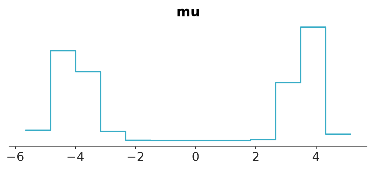
The $\widehat{R}$ values for `mu` are large and ESS values for `mu` are small indicating convergence problems. The following figure shows the histogram and trace plots of the posterior draws, clearly showing the bimodality and that chains are not mixing between the modes.
```{python}
#| label: fig-bimodal1_hist
az.plot_dist(
    dt_tt,
    kind="hist",
    visuals={
        "point_estimate": False,
        "point_estimate_text": False,
        "credible_interval": False,
    },
)
```
In this toy example, with random initialization each chain has
50\% probability of ending in either mode. We used Stan's default of 4 chains, and when random initialization is used, there is 6\% chance that when running Stan once, we would miss the
multimodality. If the attraction areas within the random
initialization range are not equal, the probability of missing one
mode is even higher. There is a tradeoff between the default
computation cost and cost of having higher probability of finding
multiple modes. If there is a reason to suspect multimodality, it
is useful to run more chains. Running more chains helps to diagnose
the multimodality, but the probability of chains ending in
different modes can be different from the relative probability mass
of each mode, and running more chains doesn't fix this. Other means
are needed to improve mixing between the modes (e.g. Yao et al.,
2020) or to approxima|tely weight the chains (e.g. Yao et al.,
2022).
## Easy bimodal posterior
If the modes in the bimodal distribution are not strongly
separated, MCMC can jump from one mode to another and there are no
convergence issues.
```{python}
N = 20
y = np.concatenate([rng.normal(-3, 1, N // 2), rng.normal(3, 1, N // 2)])
data_tt = {"N": N, "y": y}
```
```{python}
#| label: fit_tt_easy
fit_tt = mod_tt.sample(data=data_tt, seed=SEED, show_progress=False)
dt_tt = az.from_cmdstanpy(fit_tt)
```
### Convergence diagnostics
We check the diagnostics
```{python}
az.diagnose(dt_tt)
```
```{python}
az.summary(dt_tt)
```
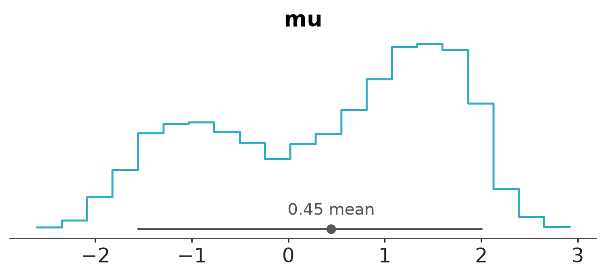
Two modes are visible.
```{python}
#| label: fig-bimodal2_hist
az.plot_dist(dt_tt, kind="hist")
```
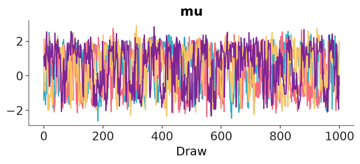
Trace plot is not very useful. It shows the chains are jumping between modes, but it's difficult to see whether the jumps happen often enough and chains are mixing well.
```{python}
#| label: fig-bimodal2_trace
az.plot_trace(dt_tt);
```
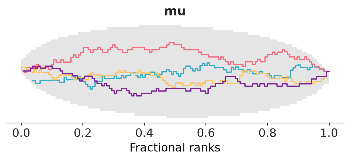
Rank plot [@Sailynoja+etal:2022:PIT-ECDF] indicates good mixing as all chains have their lines inside the envelope. The envelope assumes no autocorrelation, hence `az.plot_rank` automatically thins the draws here. This can be disable by passing the argument.`thin=False`.
```{python}
#| label: fig-bimodal2_rank
az.plot_rank(dt_tt)
```
## Initial value issues
MCMC requires some initial values. By default, Stan generates them randomly from [-2,2] in unconstrained space (constraints on parameters are achieved by transformations). Sometimes these initial values can be bad and cause numerical issues. Computers,(in general) use finite number of bits to present numbers and with very small or large numbers, there can be problems of presenting them or there can be significant loss of accuracy.
The data is generated from a Poisson regression model. The Poisson intensity parameter has to be positive and usually the latent linear predictor is exponentiated to be positive (the exponentiation can also be justified by multiplicative effects on Poisson intensity).
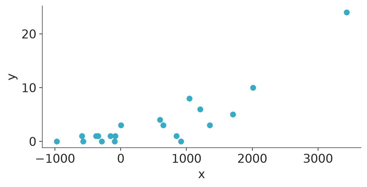
We intentionally generate the data so that there are initialization problems, but the same problem is common with real data when the scale of the predictors is large or small compared to the unit scale. The following figure shows the simulated data.
### Data
```{python}
np.random.seed(SEED + 6)
M = 1
N = 20
x = 1e3 * np.sort(np.random.randn(N)).reshape(-1, M)
y = np.random.poisson(np.exp(1e-3 * x[:, 0]))
data_pois = {"M": M, "N": N, "x": x, "y": y}
```
```{python}
#| label: fig-poisson_data
_, ax = plt.subplots(figsize=(6, 3))
ax.scatter(x, y)
ax.set(xlabel='x', ylabel='y');
```
### Model
We use a Poisson regression model with proper priors. The
`poisson_log_glm` corresponds to a distribution in which the log intensity of the Poisson distribution is modeled with `alpha + beta * x` but is implemented with better computational efficiency.
```{python}
mod_pois = CmdStanModel(stan_file="pois_glm.stan")
print_stan(mod_pois)
```
Sample
```{python}
#| label: fit_pois
mod_pois = CmdStanModel(stan_file="pois_glm.stan")
fit_pois = mod_pois.sample(data=data_pois, seed=SEED, show_progress=False)
dt_pois = az.from_cmdstanpy(fit_pois)
```
We get a lot of warnings about rejecting initial values.
### Convergence diagnostics
We check the diagnostics:
```{python}
az.diagnose(dt_pois)
```
```{python}
dt_pois = az.from_cmdstanpy(fit_pois)
az.summary(dt_pois)
```
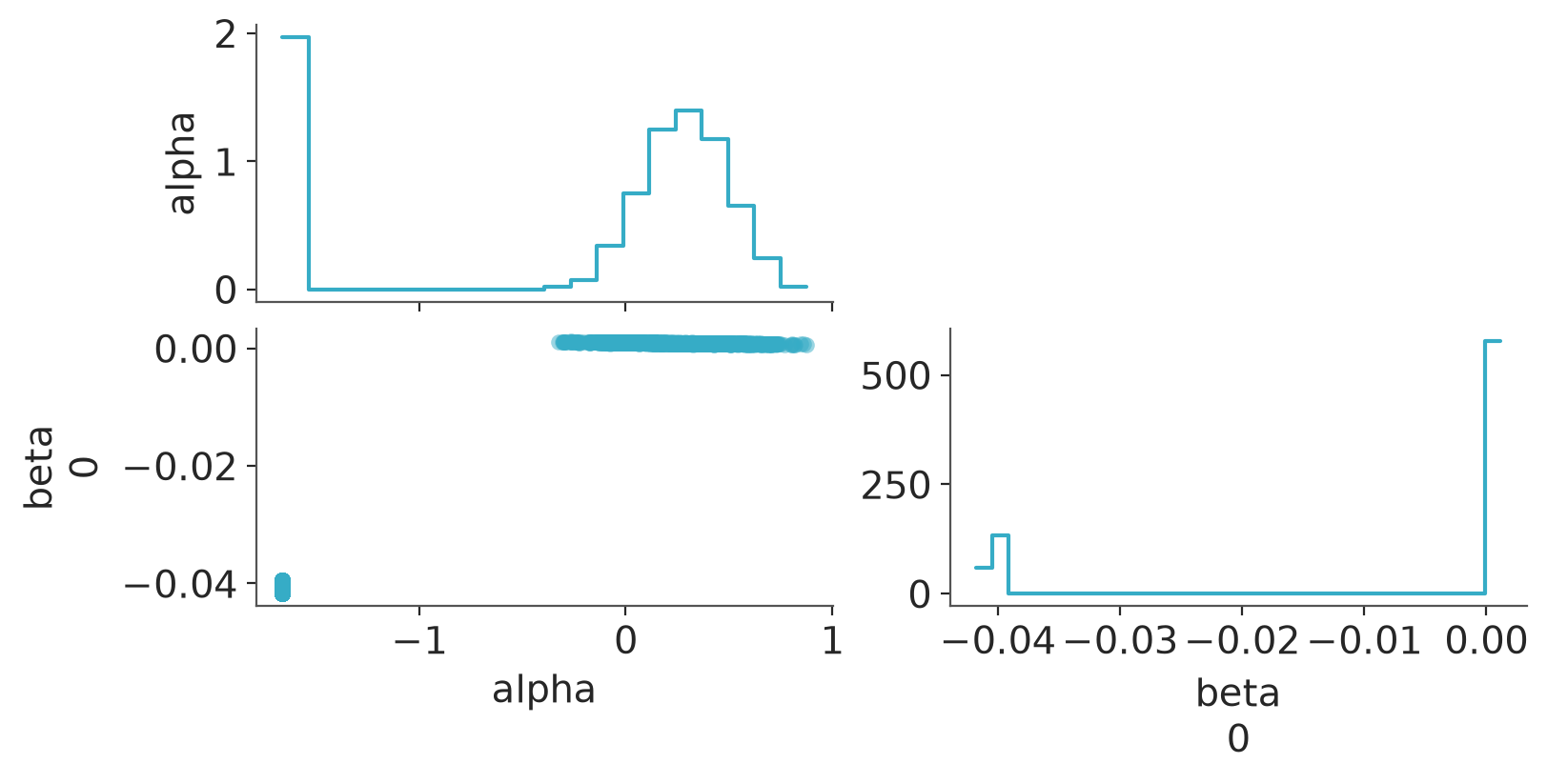
$\widehat{R}$ values are large and ESS values are small, indicating bad mixing. Marginal histograms and joint scatterplots of the posterior draws in the figure below clearly show that two chains have been stuck away from two others.
```{python}
#| label: fig-poisson_pairs
az.plot_pair(
    dt_pois,
    marginal_kind="hist",
    figure_kwargs={"figsize": (8, 4)},
    visuals={"divergence": True},
)
```
The reason for the issue is that the initial values for
`beta` are sampled from $(-2, 2)$ and `x` has some
large values. If the initial value for `beta` is higher than
about 0.3 or lower than $-0.4$, some of the values of
`exp(alpha + beta * x)` will overflow to floating point
infinity (`Inf`).
### Scaled data
Sometimes an easy option is to change the initialization range. For
example, in this case the sampling succeeds if the initial values are
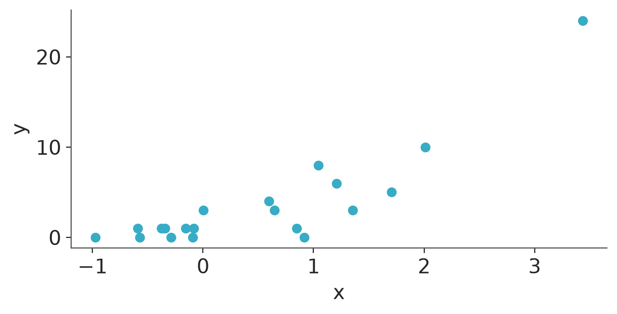
drawn from the range $(-0.001, 0.001)$. Alternatively we can scale
`x` to have scale close to unit scale. After this scaling, the
computation is fast and all convergence diagnostics look good.
```{python}
data_pois = {'M': M, 'N': N, 'x': x / 1e3, 'y': y}
```
```{python}
#| label: fig-poisson_data2
_, ax = plt.subplots(figsize=(6, 3))
ax.scatter(data_pois["x"], data_pois["y"])
ax.set(xlabel="x", ylabel="y")
```
```{python}
#| label: fit_pois_scaled_data
fit_pois = mod_pois.sample(data=data_pois, seed=SEED, show_progress=False)
dt_pois = az.from_cmdstanpy(fit_pois)
```
### Convergence diagnostics
We check the diagnostics:
```{python}
az.diagnose(dt_pois)
```
```{python}
az.summary(dt_pois)
```
If the initial value warning comes only once, it is possible that MCMC was able to escape the bad region and rest of the inference is ok.
## Thick tailed posterior
We return to the logistic regression example with separable data. Now we use proper, but thick tailed Cauchy prior.
### Model
```{python}
#| output: asis
mod_logit_glm4 = CmdStanModel(stan_file="logit_glm4.stan")
print_stan(mod_logit_glm4)
```
Sample
```{python}
#| label: fit_logit_glm4
np.random.seed(SEED + 4)
M = 1
N = 10
x = np.sort(np.random.randn(N)).reshape(-1, M)
y = np.repeat([0, 1], N // 2)
data_logit = {"M": M, "N": N, "x": x, "y": y}

fit_logit_glm4 = mod_logit_glm4.sample(data=data_logit, seed=SEED, show_progress=False)
dt_logit_glm4 = az.from_cmdstanpy(fit_logit_glm4)
```
### Convergence diagnostics
We check diagnostics
```{python}
az.diagnose(dt_logit_glm4)
```
```{python}
az.summary(dt_logit_glm4)
```
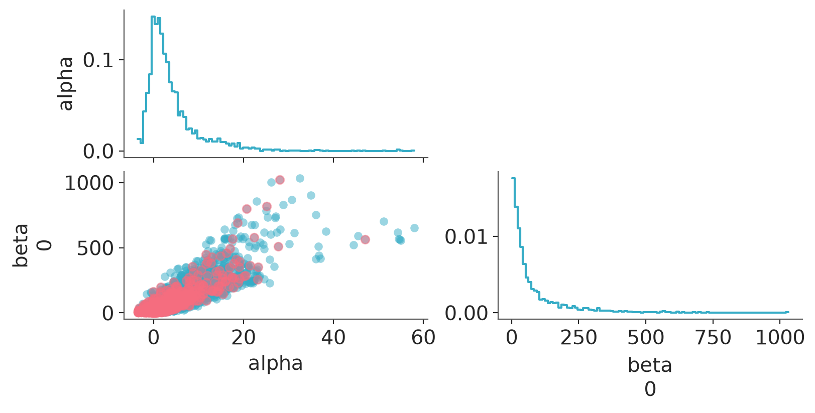
The rounded $\widehat{R}$ values look good, ESS values are low. Looking at the marginal histograms and joint scatterplots of the posterior draws in the following figure show a thick tail.
```{python}
#| label: fig-thick_tail_pairs
az.plot_pair(
    dt_logit_glm4,
    marginal_kind="hist",
    figure_kwargs={"figsize": (8, 4)},
    visuals={"divergence": True},
)
```
The dynamic HMC algorithm used by Stan, along with many other MCMC methods, have problems with such thick tails and mixing is
slow.
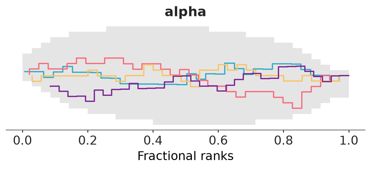
Rank plot indicates good mixing as all chains have their lines inside the envelope. The envelope assumes no autocorrelation, hence `az.plot_rank` automatically thins the draws here. This can be disable by passing the argument.`thin=False`. Notice how the envelope looks highly stepped/jagged; because heavy thinning (due to low ESS) leaves so few draws to compute the rank plots and its envelope.
```{python}
#| label: fig-thick_tail_rank
az.plot_rank(dt_logit_glm4, var_names=["alpha"])
```
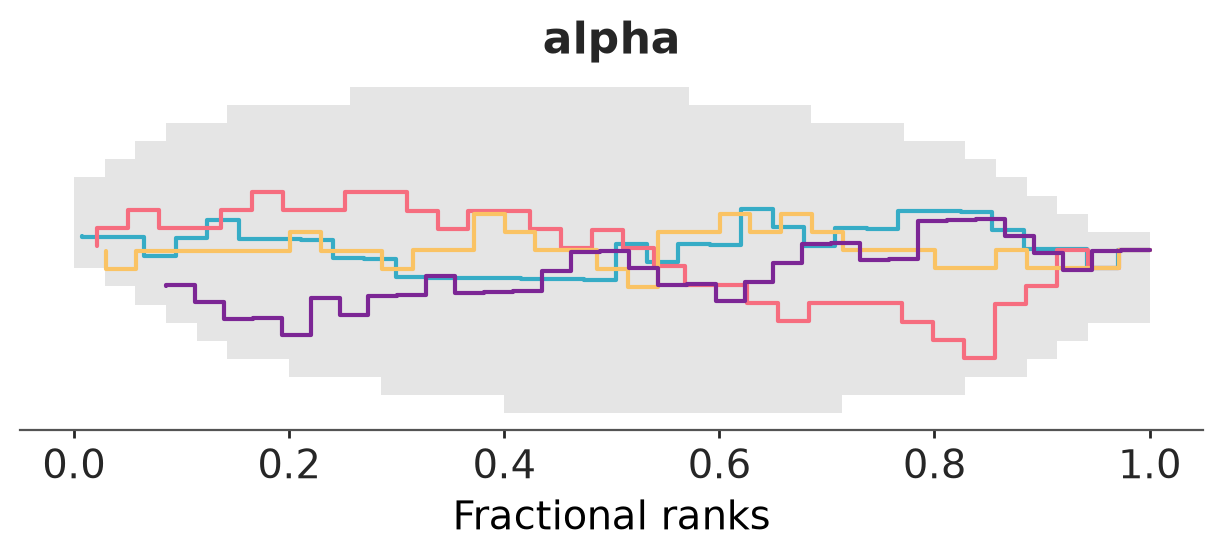
More iterations confirm a reasonable mixing.
```{python}
fit_logit_glm4 = mod_logit_glm4.sample(
    data=data_logit,
    seed=SEED,
    show_progress=False,
    iter_sampling=4000
)
```
```{python}
idata_logit_glm4 = az.from_cmdstanpy(fit_logit_glm4)
az.summary(idata_logit_glm4)
```
```{python}
#| label: fig-thick_tail_rank_more
az.plot_rank(dt_logit_glm4, var_names=["alpha"])
```
## Variance parameter that is not constrained to be positive
Demonstration what happens if we forget to constrain a parameter
that has to be positive. In Stan the constraint can be added when
declaring the parameter as `real<lower=0> sigma;`
### Data
We simulated x and y independently from normal(0,1) and normal(0,0.1)
respectively. As $N=8$ is small, there will be a lot of uncertainty
about the parameters including the scale sigma.
```{python}
M = 1
N = 8
np.random.seed(SEED)
x = np.random.randn(N).reshape(-1, M)
y = np.random.randn(N) / 10
data_lin = {'M': M, 'N': N, 'x': x, 'y': y}
```
### Model
We use linear regression model with proper priors.
```{python}
mod_lin = CmdStanModel(stan_file="linear_glm.stan")
print_stan(mod_lin)
```
Sample
```{python}
#| label: fit_lin
fit_lin = mod_lin.sample(data=data_lin, seed=SEED, show_progress=False)
idata_lin = az.from_cmdstanpy(fit_lin)
```
We get many warnings about the scale parameter being negative.
Sometimes these warnings appear in early phase of the sampling,
even if the model has been correctly defined. Now we have too many
of them, which indicates the sampler is trying to jump to
infeasible values, which here means the negative scale parameter
values. Many rejections may lead to biased estimates.
There are some divergences reported, which is also indication that
there might be some problem (as divergence diagnostic has an ad hoc
diagnostic threshold, there can also be false positive
warnings). Other convergence diagnostics are good, but due to many
rejection warnings, it is good to check the model code and
numerical accuracy of the computations.
### Convergence diagnostics
We check diagnostics
```{python}
az.diagnose(idata_lin)
```
```{python}
az.summary(idata_lin)
```
### Stan compiler pedantic check
Stan compiler pedantic check can recognize that a normal distribution
is given parameter sigma as a scale parameter, but sigma was not
constrained to be strictly positive. The pedantic check is also warning
about the very wide priors.
After fixing the model with proper parameter constraint, MCMC runs
without warnings and the sampling efficiency is better. In this
specific case, the bias is negligible when running MCMC with the
model code without the constraint, but it is difficult to diagnose
without running the fixed model.
Fixed model includes `<lower=0>` constraint for sigma.
```{python}
mod_lin2 = CmdStanModel(stan_file="linear_glm2.stan")
print_stan(mod_lin2)
```
Sample
```{python}
#| label: fit_lin2
fit_lin2 = mod_lin2.sample(data=data_lin, seed=SEED, show_progress=False)
```
We check diagnostics
```{python}
idata_lin2 = az.from_cmdstanpy(fit_lin2)
az.summary(idata_lin2)
```
In this specific case, the bias is negligible when running MCMC
with the model code without the constraint, but it is difficult to
diagnose without running the fixed model.
<br />
## References {.unnumbered}
<div id="refs"></div>
## Licenses {.unnumbered}
* Code © 2021--2025, Aki Vehtari, licensed under BSD-3.
* Text © 2021--2025, Aki Vehtari, licensed under CC-BY-NC 4.0.