10 Prior Elicitation
Specification of the prior distribution for a Bayesian model is key, but it is often difficult even for statistical experts. Having to choose a prior distribution is portrayed both as a burden and as a blessing. We choose to affirm that is a necessity, if you are not choosing your priors someone else is doing it for you (Mikkola et al. 2024). Letting others decide for you is not always a bad idea. Default priors provided by tools like Bambi or brms can be very useful in many problems, but it’s advantageous to be able to specify custom priors when needed.
The process of transforming domain knowledge into well-defined prior distributions is called Prior Elicitation and as we already said is an important part of Bayesian modelling. In this chapter, we will discuss some general approaches to prior elicitation and provide some examples. Two other sources of information about prior elicitation that complement this chapter are the PreliZ documentation, a Python package for prior elicitation that we will discuss here, and PriorDB, a database of prior distributions for Bayesian analysis.
10.1 Priors and Bayesian Statistics
If you are reading this guide, you probably already know what a prior distribution is. But let’s do a quick recap. In Bayesian statistics, the prior distribution is the probability distribution that expresses information about the parameters of the model before observing the data. The prior distribution is combined with the likelihood to obtain the posterior distribution, which is the distribution of the parameters after observing the data.
Priors are one way to convey domain-knowledge information into models. Other ways to include information in a model are the type of model or its overall structure, e.g. using a linear model, and the choice of likelihood.
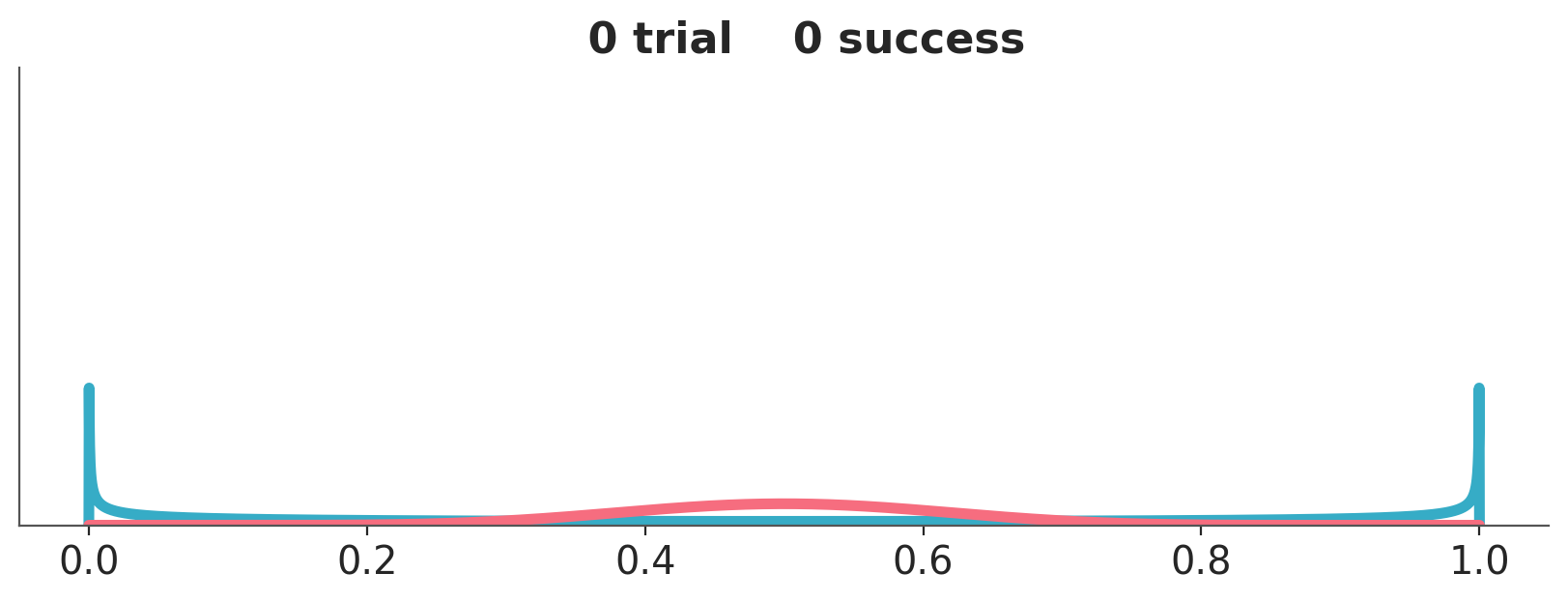
Let use a couple of examples to think about priors and it’s role in Bayesian statistics, Figure 10.2 shows two priors, one in blue (Beta(0.5, 0.5)) and one in red (Beta(10, 10)).
We are going to combine these priors with data using a Binomial likelihood. And we are going to update these priors sequentially, i.e. we will be adding some data and compute the posterior. And then add some more data and keep updating. So, at each step \(i\) we add data and the distribution we are computing are the posteriors, but these posteriors are also the priors for step \(i+1\). This sequential updating, where a posterior becomes the prior of the next analysis, is possible because the Beta distribution is conjugate with the Binomial. Conjugate prior are priors that when combined with a likelihood function result in a posterior distribution that is of the same form as the prior distribution. Usually, we don’t care too much about conjugate priors, but sometimes, like for this animation, they can be useful.
We have represented these sequential updating in an animation (see Figure 10.3). As the animation moves forward, i.e. we add more data, we will see that the posteriors gradually converge to the same distribution.
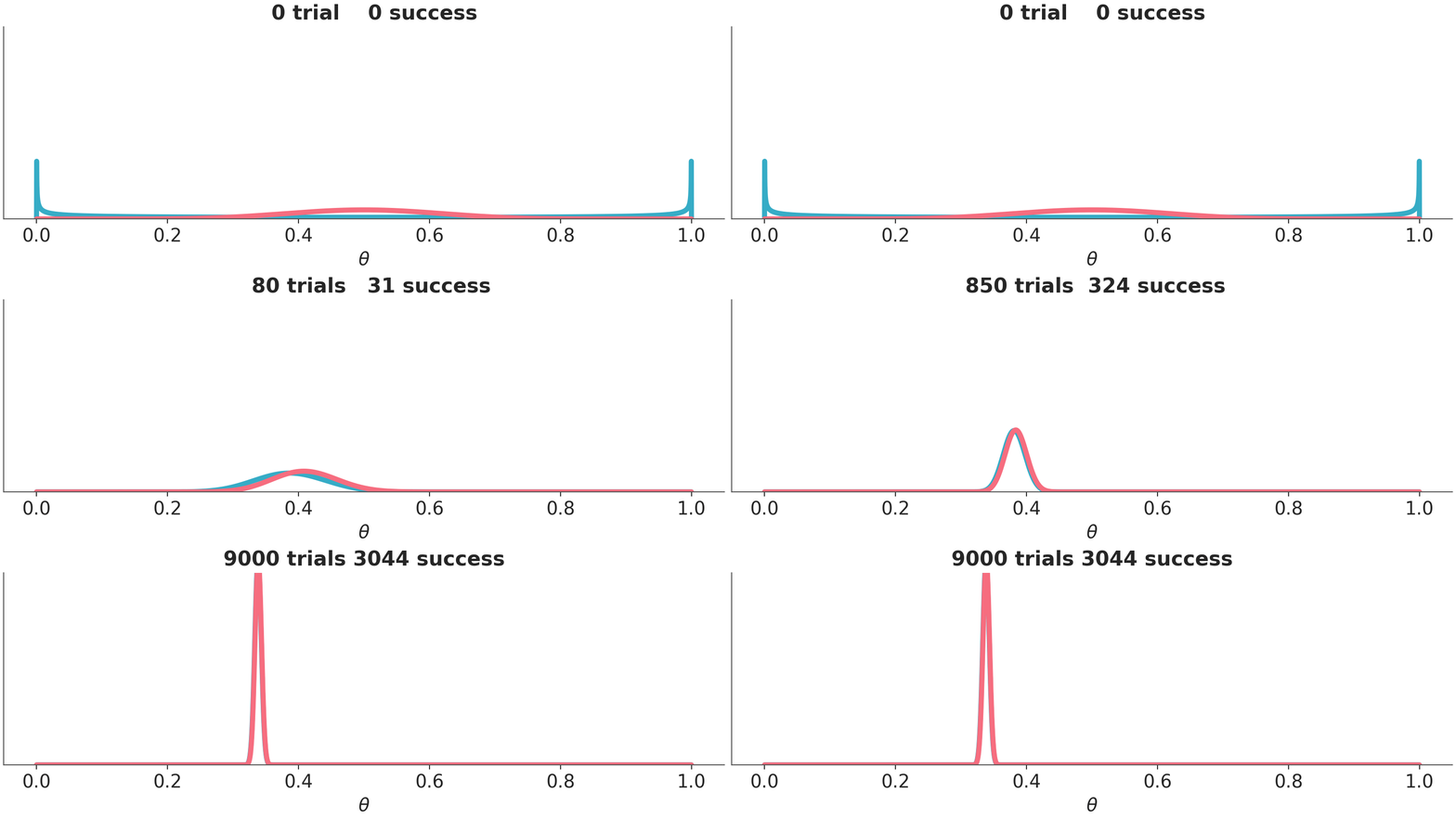
Asymptotically, priors have no meaning. If we have infinite data, the posterior will be the same regardless of the chosen prior. When there is large amount of data, the update is dominated by the likelihood function, and the prior has little influence. Different reasonable priors converge to the same posterior as data size is increased.
But there are two catches. If we assign 0 prior probability to a value, no amount of data will turn that into a positive value. In other words, if a particular value or hypothesis is assigned zero prior probability, it will also have zero posterior probability, regardless of the data observed. Alternatively, if we assign a prior probability of 1 to a value (and zero to the rest), no amount of data will allow us to update that prior neither. This is known as Cromwell’s rule and states that the use of prior probabilities of 1 (“the event will definitely occur”) or 0 (“the event will definitely not occur”) should be avoided, except when applied to statements that are logically true or false, such as \(2+2=4\).
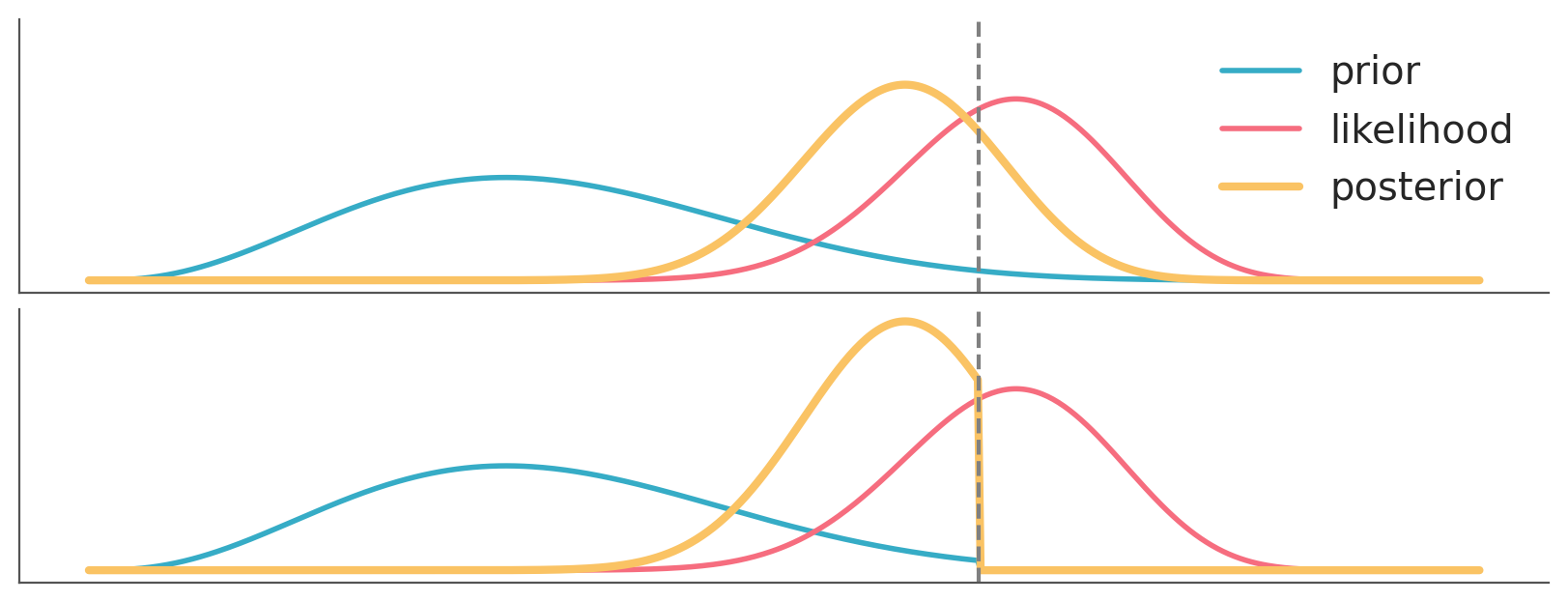
OK, but if we take Cromwell’s advice and avoid these corner cases eventually the data will dominate the priors. That’s true, as well as that asymptotically, we are all dead. For real, finite data, we should expect priors to have some impact on the results. The actual impact will depend on the specific combinations of priors, likelihood and data. Section 10.3 shows a couple of combinations. In practice we often need to worry about our priors, but maybe less than we think.

10.2 Types of Priors
Usually, priors are described as informative vs non-informative. Informative priors are priors that convey specific information about the parameters of the model, while non-informative priors do not convey specific information about the parameters of the model. Non-informative priors are often used when little or no domain knowledge is available. A simple, intuitive and old rule for specifying a non-informative prior is the principle of indifference, which assigns the same probability to all possible events. Non-informative priors are also called objective priors especially when the main motivation for using them is to avoid the need to specify a prior distribution.
Non-informative priors can be detrimental and difficult to implement or use. Informative priors can also be problematic in practice, as the information needed to specify them may be absent or difficult to obtain. And even if the information is available specifying informative priors can be time-consuming. A middle ground is to use weakly informative priors, which are priors that convey some information about the parameters of the model but are not overly specific. Weakly informative priors can help to regularize inference and even have positive side effects like improving sampling efficiency.
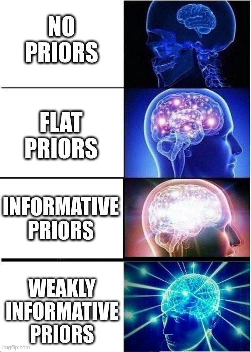
It is important to recognize that the amount of information a priors carry can vary continuously and that the categories we use to discuss priors are a matter of convenience and not a matter of principle. These categories are qualitative and not well-defined. Still, they can be helpful when talking about priors more intuitively.
So far we have discussed the amount of information. There are at least two issues that seem fishy about this discussion. First, the amount of information is a relative concept, against what are we evaluating if a prior is informative or not? Second, the amount of information does not necessarily mean the information is good or correct. For instance, it’s possible to have a very informative prior based on wrong assumptions. Thus when we say informative we don’t necessarily mean reliable or that the prior will bias the inference in the correct direction and amount.
There is one way to frame the discussion about priors that can help to address these issues. That is to think about priors in terms of the prior predictive distribution they induce. In other words, we think about the priors in terms of their predictions about unobserved, potentially observable data. This mental scaffold can be helpful in many ways:
- First, it naturally leads us to think about priors in relation to other priors and the likelihood, i.e. it reflects the fact that we cannot understand a prior without the context of the model (Gelman, Simpson, and Betancourt 2017).
- Second, it gives us an operational definition of what we mean by vague, informative, or weakly informative prior. An informative prior is a prior that makes predictions that are about the same. A weakly informative prior is a prior that makes predictions that are somewhere in between. The distinctions are still qualitative and subjective, but we have a criteria that is context-dependent and we can evaluate during a Bayesian data analysis. Figure Figure 10.7 shows a very schematic representation of this idea.
- Third, it provides us with a way to evaluate the priors for consistency, because the priors we are setting should agree with the prior predictive distribution we imagine. For instance, if we are setting an informative prior that induces a prior predictive distribution that is narrower, shifted or very different in any other way from the one we imagine either the prior or our expectation of the prior predictive distribution is wrong. We have specified two conflicting pieces of information. Reconciling these two pieces of information does not guarantee that the prior or any other part of the model is correct, but it provides internal consistency, which is a good starting point for a model.
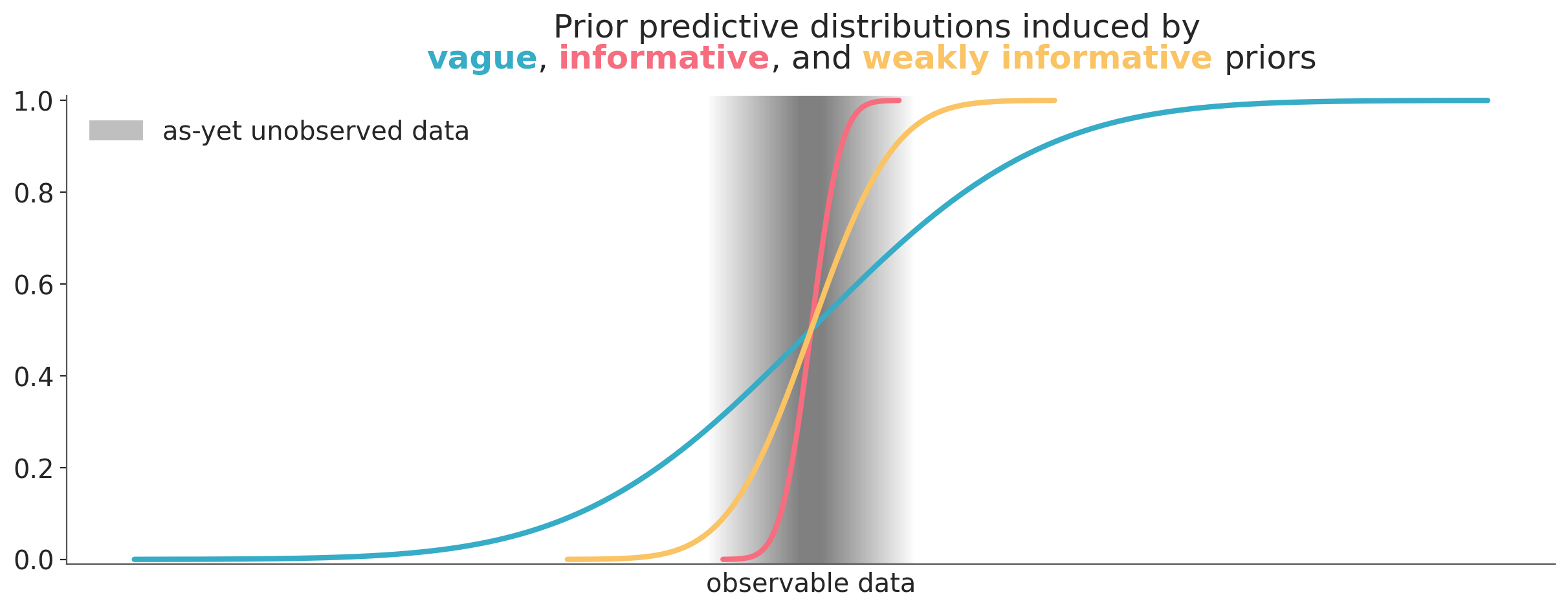
Using the prior predictive distribution to evaluate priors is inherently a global approach, as it assesses the combined impact of all priors and the likelihood. However, during prior elicitation, we may sometimes focus on making one or two priors more informative while keeping the others vague. In these cases, we can think of this as having a “local” mix of priors with varying levels of informativeness. In practice, we often balance this global perspective with the local approach, tailoring priors to the specific needs of the model.
10.3 Bayesian Workflow for Prior Elicitation
Prior elicitation is a key part of a flexible iterative workflow. It can be specific to the needs of the model and data at hand. It may need revision as we develop the model and analyse the data.
Knowing when to perform prior elicitation is central to a prior elicitation workflow. In some situations, default priors and models may be sufficient, especially for routine inference that applies the same, or very similar, model to similar new datasets. But even for new datasets, default priors can be a good starting point, adjusting them only after initial analysis reveals issues with the posterior or computational problems. As with other components of the Bayesian workflow, prior elicitation isn’t just a one-time task. It’s not even one that is always done at the beginning of the analysis.
For simple models with strong data, the prior may have minimal impact, and starting with default or weakly informed priors may be more appropriate and provide better results than attempting to generate very informative priors. The key is knowing when it’s worth investing resources in prior elicitation. Or more nuanced how much time and domain knowledge is needed in prior specification. Usually, getting rough estimates can be sufficient to improve inference. Thus, in practice, weakly informative priors are often enough. In a model with many parameters eliciting all of them one by one may be too time-consuming and not worth the effort. Refining just a few priors in a model can be sufficient to improve inference.
The prior elicitation process should also include a step to verify the usefulness of the information and assess how sensitive the results are to the choice of priors, including potential conflicts with the data. This process can help identify when more or less informative priors are needed and when the model may need to be adjusted.
Finally, we want to highlight that prior elicitation isn’t just about choosing the right prior but also about understanding the model and the problem. So even if we end up with a prior that has little impact on the posterior, compared to a vague or default prior, performing prior elicitation could be useful for the modeller. Especially among newcomers setting priors can be seen as an anxiogenic task. Spending some time thinking about priors, with the help of proper tools, can help reduce this brain drain and save mental resources for other modelling tasks.
Nevertheless, usually, the selling point when discussing in favour of priors is that they allow the inclusion of domain information. But there are potentially other advantages of :
- Sampling efficiency. Often a more informed priors results in better sampling. This does not mean we should tweak the prior distribution to solve sampling problems, instead incorporating some domain-knowledge information can help to avoid them.
- Regularization. More informed priors can help to regularize the model, reducing the risk of overfitting. We make a distinction between regularization and “conveying domain-knowledge information” because motivations and justifications can be different in each case.
10.4 Priors and entropy
The entropy is a property of probability distributions the same way the mean or variance are, actually it’s the expected value of the negative log probability of the distribution. We can think of entropy as a measure of the information or uncertainty of a distribution has. Loosely speaking the entropy of a distribution is high when the distribution is spread out and low when the distribution is concentrated. In the context of prior elicitation maximum entropy can be a guiding principle to pick priors. According to this principle we should choose the prior that maximizes the entropy, subject to known constraints of the prior (Jaynes 2003). This is a way to choose a prior that is as vague as possible, given the information we have. Figure Figure 10.8 shows a distribution with support in [0, 1]. On the first panel we have the distribution with maximum entropy and no other restrictions. We can see that this is a uniform distribution. On the middle we have the distribution with maximum entropy and a given mean. This distribution looks similar to an exponential distribution. On the last panel we have the distribution with maximum entropy and 70% of its mass between 0.5 and 0.75.

For some priors in a model, we may know or assume that most of the mass is within a certain interval. This information is useful for determining a suitable prior, but this information alone may not be enough to obtain a unique set of parameters. Figure 10.9 shows Beta distributions with 90% of the mass between 0.1 and 0.7. As you can see we can obtain very different distributions, conveying very different prior knowledge. The red distribution is the one with maximum entropy, given the constraints.

10.5 Preliz
PreliZ (Icazatti et al. 2023) is a Python package that helps practitioners choose prior distributions by offering a set of tools for the various facets of prior elicitation. It covers a range of methods, from unidimensional prior elicitation on the parameter space to predictive elicitation on the observed space. The goal is to be compatible with probabilistic programming languages (PPL) in the Python ecosystem like PyMC and PyStan, while remaining agnostic of any specific PPL.
10.6 Maximum entropy distributions with maxent
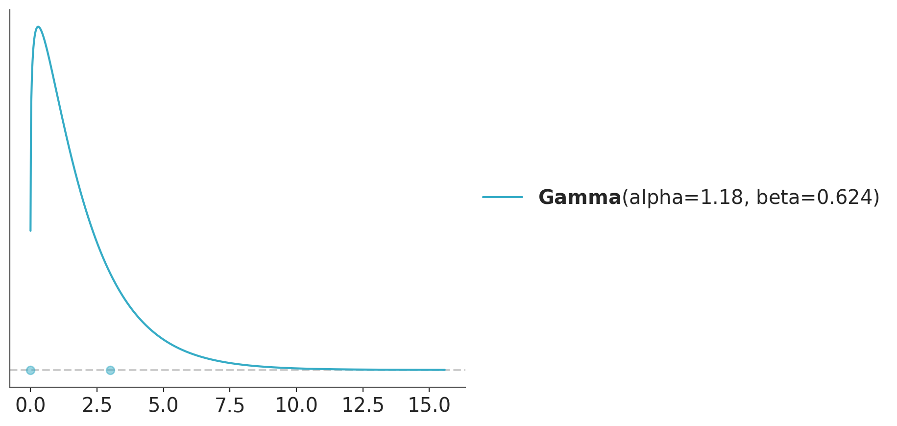
In PreliZ we can compute maximum entropy priors using the function maxent. It works for unidimensional distributions. The first argument is a PreliZ distribution. Then we specify an upper and lower bound and the probability between them.
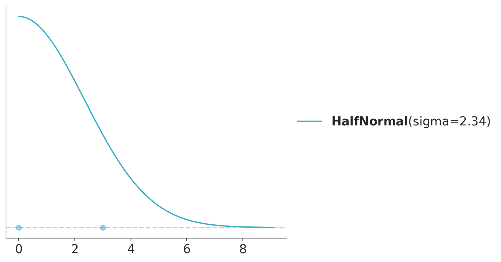
As an example, we want to elicit a scale parameter. From domain knowledge we know the parameter has a relatively high probability of being less than 3. Hence, we could use a HalfNormal distribution and do:
When we want to avoid values too close to zero, other distributions like Gamma or InverseGamma may be a better choice.
We could also have extra restrictions like knowledge about the mean or mode. Let’s say we think a mean of 2 is very likely. The Gamma distribution can be parametrized in terms of the mean as pz.Gamma(mu=2). If we instead believe the mode is likely to be 2, then maxent takes a mode argument.
dist_mean = pz.Gamma(mu=2)
pz.maxent(dist_mean, 0, 3, 0.8)

dist_mode = pz.Gamma()
pz.maxent(dist_mode, 0, 3, 0.8, mode=2);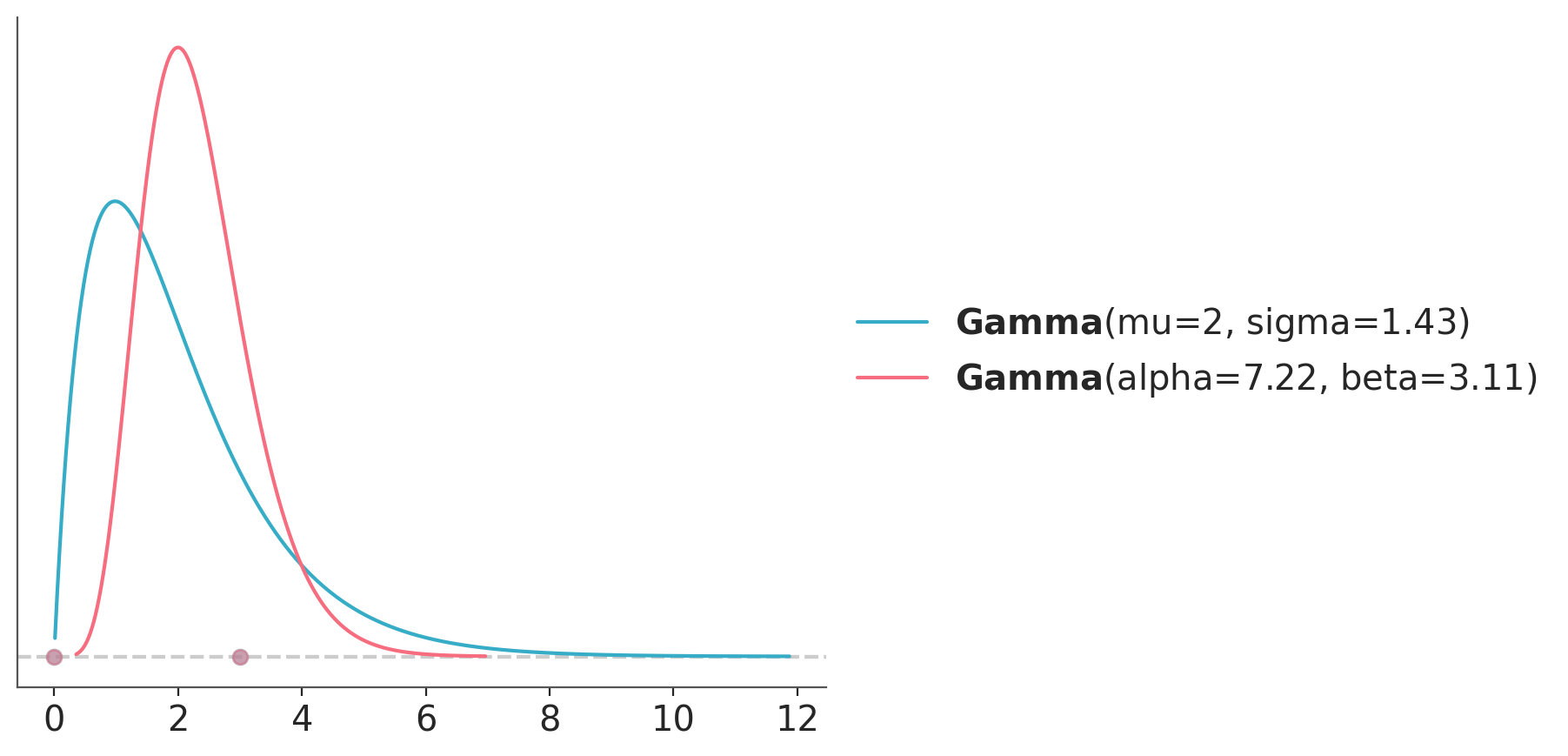
Notice that if you call maxent several times in the same cell, as we just did, we will get all the distributions in the same plot. This can be very useful to visually compare several alternatives.
The function maxent as others in PreliZ modify distribution in place, so a common workflow is to instantiate a distribution first, perform the elicitation, and then inspect its properties, plot it, or use it in some other way. For instance, we may want to check a summary of some of its properties:
/opt/hostedtoolcache/Python/3.11.11/x64/lib/python3.11/site-packages/numba/np/ufunc/dufunc.py:288: RuntimeWarning: invalid value encountered in nb_logpdf
  return super().__call__(*args, **kws)
/opt/hostedtoolcache/Python/3.11.11/x64/lib/python3.11/site-packages/numba/np/ufunc/dufunc.py:288: RuntimeWarning: invalid value encountered in nb_logpdf
  return super().__call__(*args, **kws)
(Gamma(mean=2.0, median=1.67, std=1.43, lower=0.26, upper=5.39),
Gamma(mean=2.32, median=2.22, std=0.86, lower=0.99, upper=4.19))10.7 Other direct elicitation methods from PreliZ
There are many other method for direct elicitation of parameters. For instance the quartile functions identifies a distribution that matches specified quartiles, and Quartine_int provides an interactive approach to achieve the same, offering a more hands-on experience for refining distributions.
One method worth of special mention is the Roulette method allows which allows users to find a prior distribution by drawing it interactively (Morris, Oakley, and Crowe 2014). The name “roulette” comes from the analogy of placing a limited set of chips where one believes the mass of a distribution should be concentrated. In this method, a grid of m equally sized bins is provided, covering the range of x, and users allocate a total of n chips across the bins. Effectively, this creates a histogram,representing the user’s information about the distribution. The method then identifies the best-fitting distribution from a predefined pool of options, translating the drawn histogram into a suitable probabilistic model.
As this is an interactive method we can’t show it here, but you can run the following cell to see how it works.
And this gif should give you an idea on how to use it.
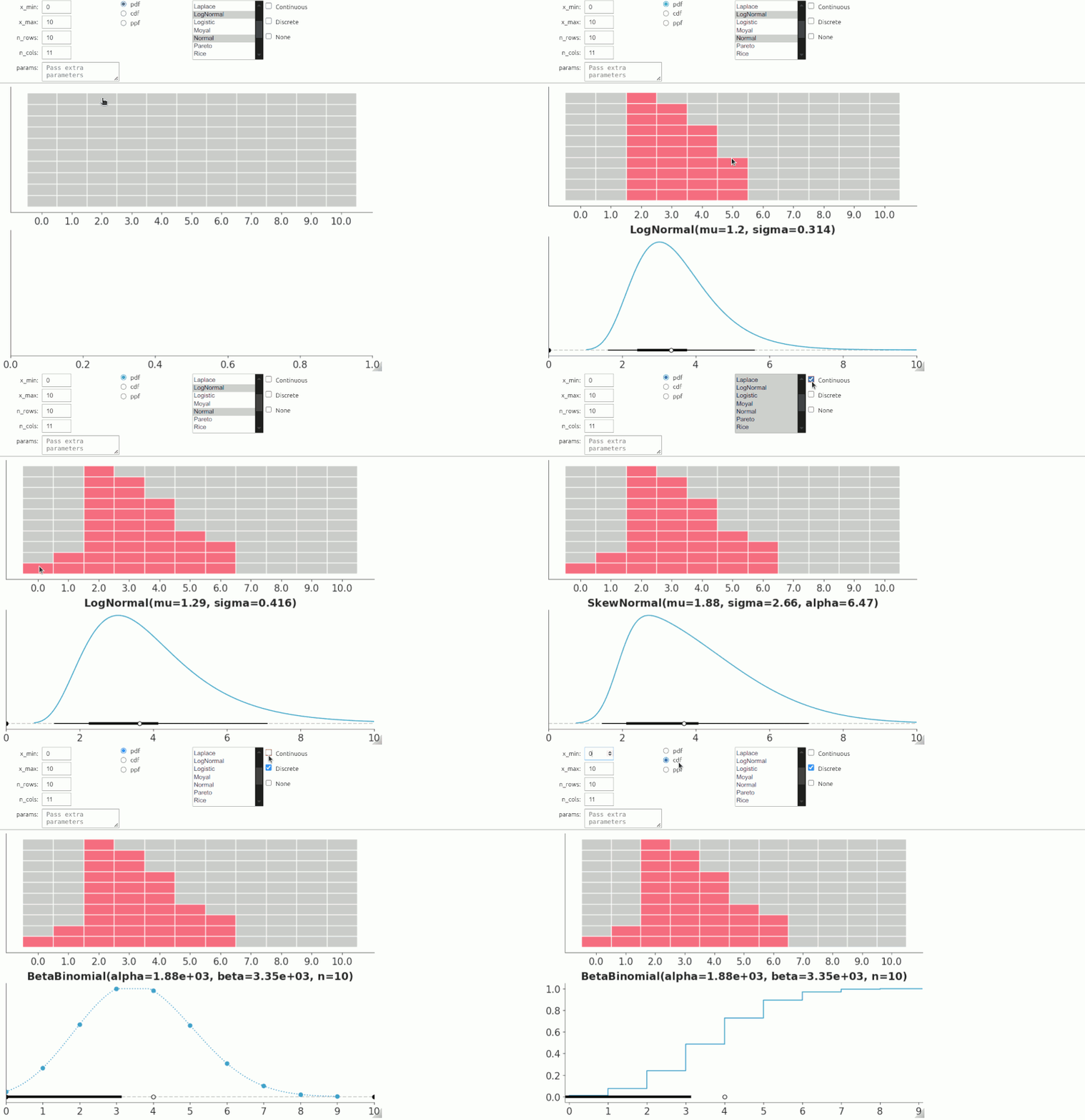
Once we have elicited the distribution we can call .dist attribute to get the selected distribution. In this example, it will be result.dist.
If needed, we can combine results for many independent “roulette sessions” with the combine_roulette function. Combining information from different elicitation sessions can be useful to aggregate information from different domain experts. Or even from a single person unable to pick a single option. For instance if we run Roulette twice, and for the first one we get result0 and for the second result1. Then, we can combine both solutions into a single one using:
In this example, we assign a larger weight to the results from the second elicitation session, we can do this to reflect uneven degrees of trust. By default, all sessions are weighted equally.
10.8 Predictive elicitation
The simplest way to perform predictive elicitation is to generate a model, sample from its prior predictive distribution and then evaluate if the samples are consistent with the domain knowledge. If there is disagreement, we can refine the prior distribution and repeat the process. This is usually known as prior predictive check and we discussed them in Chapter 5 together with posterior predictive checks.
To assess the agreement between the domain knowledge and the prior predictive distribution we may be tempted to use the observed data, as in posterior predictive checks. But, this can be problematic in many ways. Instead, we recommend using “reference values”. We can obtain a reference value from domain knowledge, like previous studies, asking clients or experts, or educated guesses. They can be typical values, or usually “extreme” values. For instance, if we are studying the temperature of a city, we may use the historical record of world temperature and use -90 as the minimum, 60 as the maximum and 15 as the average. These are inclusive values. Hence this will lead us to very broad priors. If we want something tighter we should use historical records of areas more similar to the city we are studying or even the same city we are studying. These will lead to more informative priors.
10.8.1 Predator vs prey example
We are interested in modelling the relationship between the masses of organisms that are prey and organisms that are predators, and since masses vary in orders of magnitude from a 1e-9 grams for a typical cell to a 1.3e8 grams for the blue whale, it is convenient to work on a logarithmic scale.
Let’s load the data and define the reference values.
So a model might be something like:
\[\begin{align} \mu =& Normal(\cdots, \cdots) \\ \sigma =& HalfNormal(\cdots) \\ log(mass) =& Normal(\mu, \sigma) \end{align}\]
Let’s now define a model with some priors and see what these priors imply on the scale of the data. To sample from the predictive prior we use pm.sample_prior_predictive() instead of sample and we need to define dummy observations. This is necessary to indicate to PyMC which term is the likelihood and to control the size of each predicted distribution, but the actual values do not affect the prior predictive distributions.
with pm.Model() as model:
    α = pm.Normal("α", 0, 100)
    β = pm.Normal("β", 0, 100)
    σ = pm.HalfNormal("σ", 5)
    pm.Normal("prey", α + β * pp_mass["prey_log"], σ, observed=pp_mass["predator_log"])
    idata = pm.sample_prior_predictive(samples=100)
Sampling: [prey, α, β, σ]Now we can plot the prior predictive distribution and compare it with the reference values.
ax = az.plot_ppc(idata, group="prior", kind="cumulative", mean=False, legend=False)


for key, val in refs.items():
    ax.axvline(val, ls="--", color="0.5")
    ax.text(val-7, 0.5-(len(key)/100), key, rotation=90)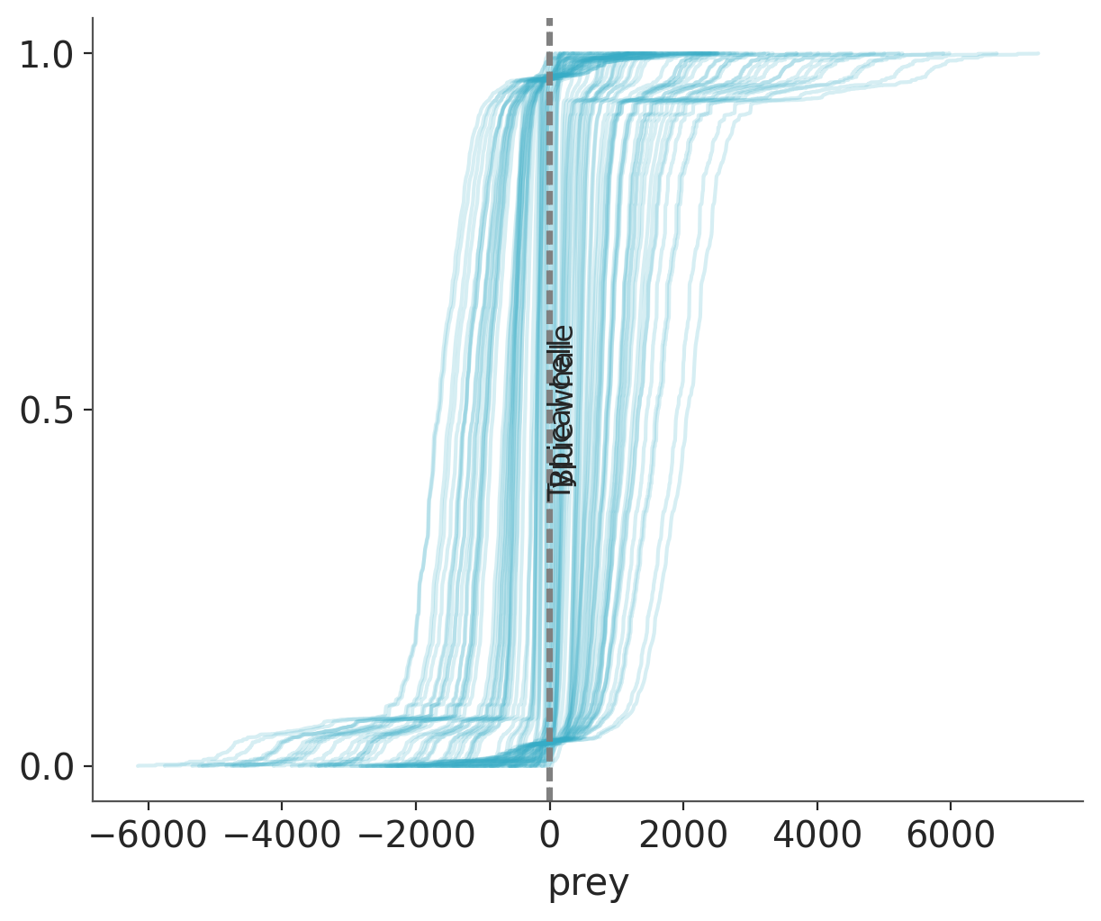
Priors are so vague that we can not even distinguish the reference values from each other. Let’s try refining our priors.
with pm.Model() as model:
    α = pm.Normal("α", 0, 1)
    β = pm.Normal("β", 0, 1)
    σ = pm.HalfNormal("σ", 5)
    prey = pm.Normal("prey", α + β * pp_mass["prey_log"], σ, observed=pp_mass["predator_log"])
    idata = pm.sample_prior_predictive(samples=100)
Sampling: [prey, α, β, σ]We can plot the prior predictive distribution and compare it with the reference values.
ax = az.plot_ppc(idata, group="prior", kind="cumulative", mean=False, legend=False)
for key, val in refs.items():
    ax.axvline(val, ls="--", color="0.5")
    ax.text(val-7, 0.5-(len(key)/100), key, rotation=90)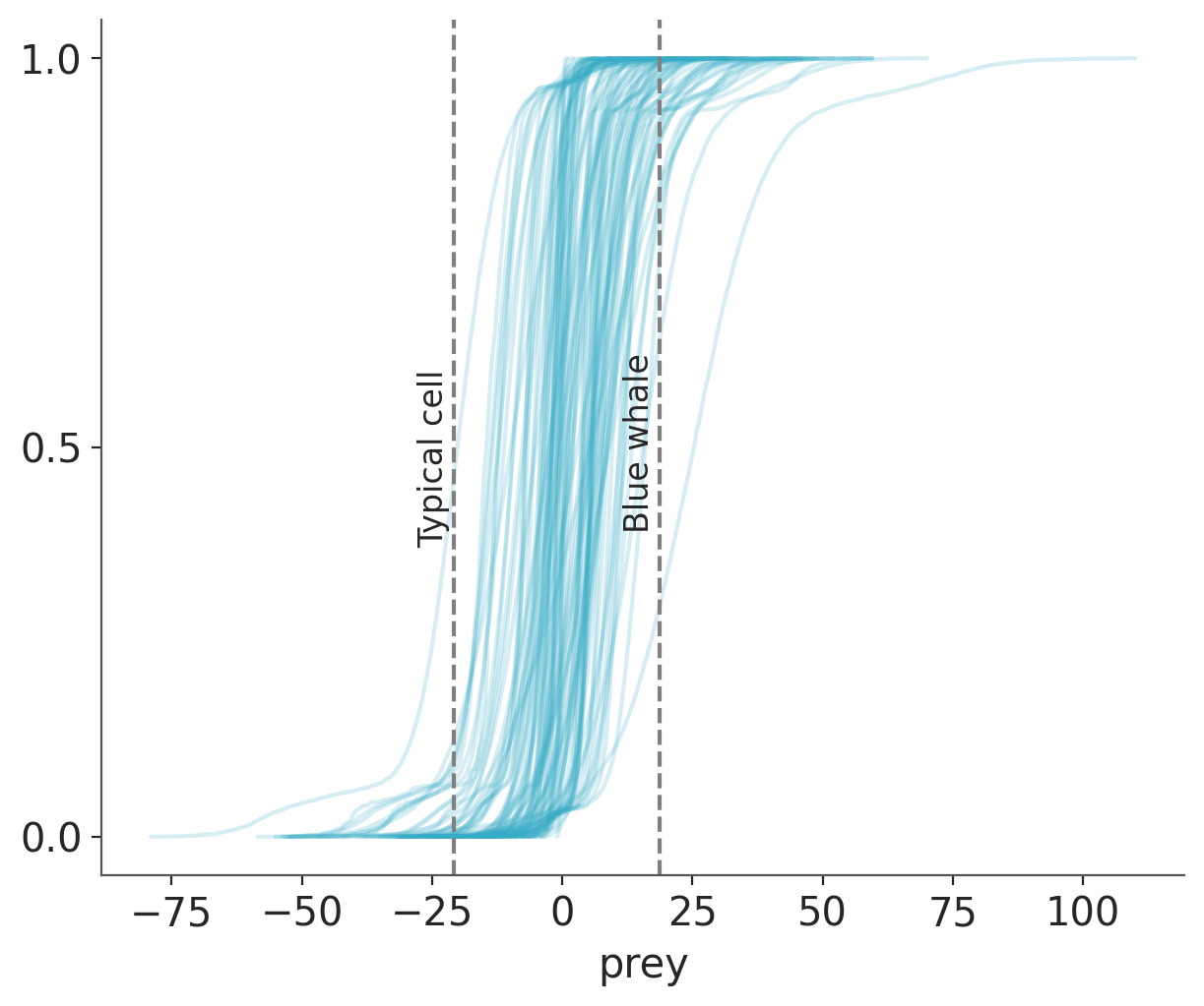
The new priors still generate some values that are too wide, but at least the bulk of the model predictions are in the right range. So, without too much effort and extra information, we were able to move from a very vague prior to a weakly informative prior. If we decided this prior is still very vague we can add more domain-knowledge.
10.8.2 Interactive predictive elicitation
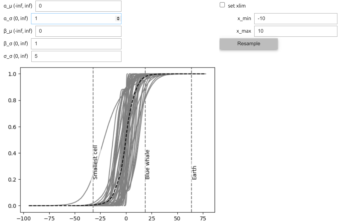
The process described in the previous section is straightforward: sample from the prior predictive –> plot –> refine –> repeat. On the good side, this is a very flexible approach and can be a good way to understand the effect of individual parameters in the predictions of a model. But it can be time-consuming and it requires some understanding of the model so you know which parameters to tweak and in which direction.
One way to improve this workflow is by adding interactivity. We can do this with PreliZ’s function, predictive_explorer. Which we can not show here, in a full glory but you can see an static image in Figure 10.11, and you can try it for yourself by running the following block of code.
10.9 Projective predictive elicitation
Projective predictive elicitation is an experimental method to elicit priors by specifying an initial model and a prior predictive distribution. Then instead of elicitate the prior themselves, we elicit the prior predictive distribution, which we call the target distribution. Then we use a procedure that automatically find the parameters of the prior that induce a prior predictive distribution that is as close as possible to the target distribution. This method is particularly useful when we have a good idea of how the data should look like, but we are not sure how to translate this into a prior distribution.
This method has been implemented in PreliZ, let see one example first and then discuss some details. To keep things concrete and familiar let’s assume we are still interested in the predator-prey example. And let assume that on a log-scale we think that the the prior predictive distribution is well described as a Normal distribution with most of its mass between the weight of a typical cell and the weight of a blue whale. The Normal is easy to work with and with this information we could derive its parameter. But let do something even easier. Let use pz.maxent and translate “most of it mass” to \(0.94\).
This will be our target distribution. If for a particular problem you are unsure about what distribution to choose as a target, think that this should be the distribution that you expect to match in a prior predictive check as discussed in previous sections. And also think that usually the goal is to find a weakly informative prior. So, the target will usually be a very approximate distribution.
Now that we have the target, we write a model as you would do before a prior predictive check, we can reuse the model from previous section. The we pass the model and target to ppe
with pm.Model() as model:
    α = pm.Normal("α", 0, 100)
    β = pm.Normal("β", 0, 100)
    σ = pm.HalfNormal("σ", 5)
    prey = pm.Normal("prey", α + β * pp_mass["prey_log"][:100], σ, observed=pp_mass["predator_log"][:100])

print(pz.ppe(model, target))
/opt/hostedtoolcache/Python/3.11.11/x64/lib/python3.11/site-packages/preliz/predictive/ppe.py:59: UserWarning: This method is experimental and under development with no guarantees of correctness.
Use with caution and triple-check the results.
warnings.warn(with pm.Model() as model:
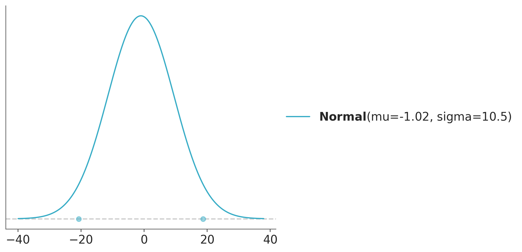
α = pm.Normal("α", mu=-0.997, sigma=1.13)
β = pm.Normal("β", mu=-0.00669, sigma=0.168)
σ = pm.HalfNormal("σ", sigma=10.3)
OK, ppe function returns a solution, because this is an experimental method, and because good data analysis always keep a good dose of scepticism of their tools, let’s check that the suggested prior is reasonable given the provided information. To do this we write the model with the new prior and sample from the prior predictive. Notice that we could have copied the priors verbatim, but instead we are rounding them. We do not care of the exact solution, a rounded number is easier to read. Feel free to not follow suggestion from machine blindly or be prepared to end inside a lake.
with pm.Model() as model:
    α = pm.Normal("α", mu=-1, sigma=1.1)
    β = pm.Normal("β", mu=0.015, sigma=0.2)
    σ = pm.HalfNormal("σ", sigma=10)
    prey = pm.Normal("prey", α + β * pp_mass["prey_log"], σ, observed=pp_mass["predator_log"])
    idata = pm.sample_prior_predictive()
Sampling: [prey, α, β, σ]Now we can plot the prior predictive distribution, the target distribution and compare it with the reference values.
ax = az.plot_ppc(idata, group="prior", kind="cumulative", mean=False, legend=False)
target.plot_cdf(color="C1")

for key, val in refs.items():
    ax.axvline(val, ls="--", color="0.5")
    ax.text(val-7, 0.5-(len(key)/100), key, rotation=90)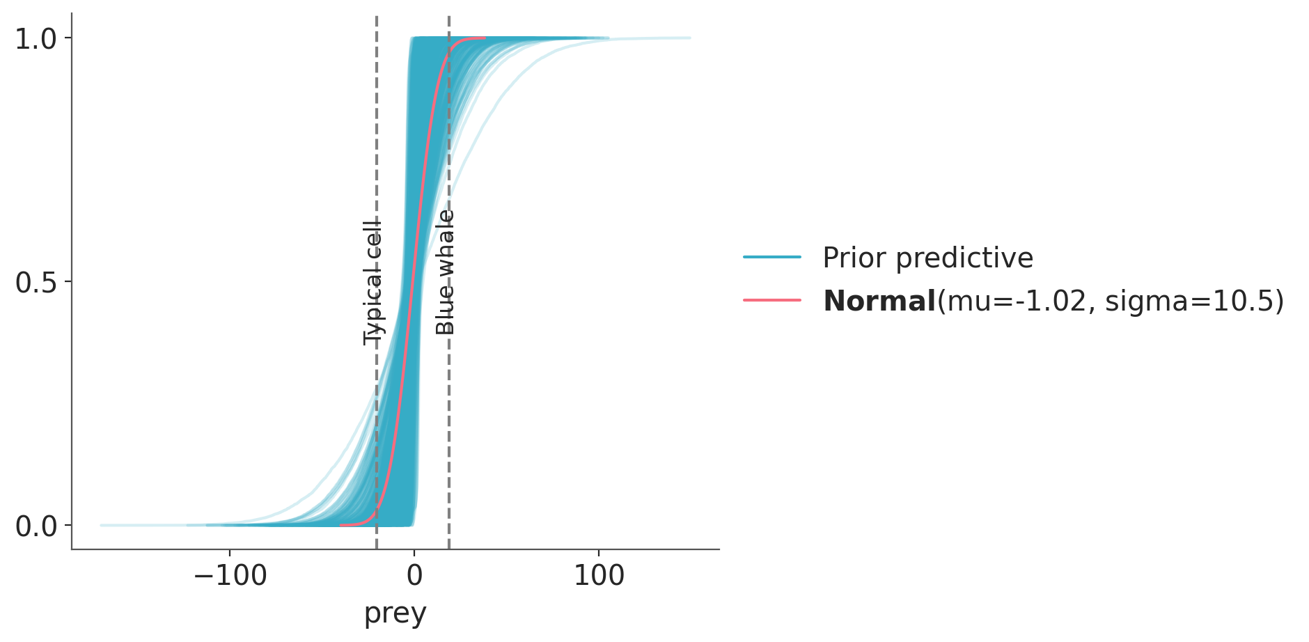
We see very good agreement. Let’s do one more plot. This time we hide the individual prior predictive samples and instead plot the aggregated prior predictive distribution, labelled with “mean” as it is the average distribution when we average over all the computed prior predictive distributions.
ax = az.plot_ppc(idata, group="prior", kind="cumulative", mean=True, legend=False, alpha=0.001)
target.plot_cdf(color="black")

for key, val in refs.items():
    ax.axvline(val, ls="--", color="0.5")
    ax.text(val-7, 0.5-(len(key)/100), key, rotation=90)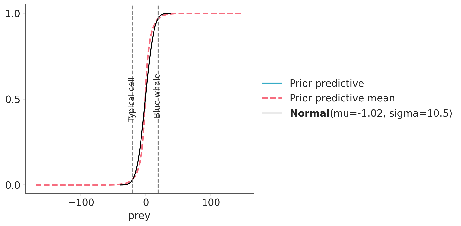
As before we point out that this prior is still relatively vague, and we could use more information to tighten up. But what we care at this point is that the prior we got is consistent with the target distribution, and thus a prior that is coherent the domain-knowledge information that we decide to use.
10.9.1 OK, but what’s under the hood?
The main idea is that once we have a target distribution we can define the prior elicitation problem as finding the parameters of the model that induce a prior predictive distribution as close as possible to the target distribution. Stated this way, this is a typical inference problem that could be solved using standard (Bayesian) inference methods that instead of conditioning on observed data we condition on synthetic data, our target distribution. Conceptually that’s what ppe is doing, but we still have two plot twist ahead of us.
The procedure is as follows:
- Generate a sample from the target distribution.
- Maximize the model’s likelihood wrt that sample (i.e. we find the parameters for a fixed “observation”).
- Generate a new sample from the target distribution and find a new set of parameters.
- Collect the parameters, one per prior parameter in the original model.
- Use MLE to fit the optimized values to their corresponding families in the original model.
Instead of using standard inference methods like MCMC in step 1-3 we are using projection inference. See Chapter 9 for details. Essentially we are approximating a posterior using an optimization method. Yes, we say posterior, because from the inference point we are computing a posterior, once that we then will use as prior. On the last step, we use a second approximation, we fit the projected posterior into standard distributions used by PPLs as building blocks. We need to do this so we can write the resulting priors in terms a PPLs like PyMC, PyStan could understand.
This procedure ignores the prior information in the model passed to ppe, because the optimized function is just the likelihood. In the last step we use the information about each prior families. But in principle, we could even ignore this information and fit the optimized values to many families and pick the best fit. This allows the procedure to suggest alternative families. For instance, it could be that we use a Normal for a given parameters but the optimization only found positive values so a Gamma or HalfNormal could be a better choice. Having said that, the prior can have an effect because they are used to initialize the optimization routine. But for that to happen the prior has to be very off with respect to the target. Internally ppe performs many optimizations each time for a different sample from the target, the result of one optimization is stored as one projected posterior “sample” and also used as the initial guess for the next one. For the very first optimization, the one initialized from the prior, the result is discarded and only used as the initial guess for the next step.Another piece of information that is ignored is the observed data, the procedure only takes into account the sample size, but not the actual values. So you can pass dummy values, changing the sample size can we used to obtain more narrow (larger sample size) or more vague (smaller sample size) priors. Whether we should always use the same sample size of the data we are going to actually use or not is something that needs further research and evaluation.
